
Quantum Computing is an emerging technology. Once thought to be several decades away from conception, massive interest by nation states and international corporations obtaining superior computer power has driven this field to an arguably premature fruition.
However, the rapid increase in the interest in quantum computation. has created some very different physical engineering concepts in obtaining it.
A little history helps move things along sometimes. Where did the concept of a quantum computer come from, why are they even necessary? Although computers have formidable power, it was clear even in their early days that they could not simulate the effects of quantum mechanics very well.
Since simulations are how physics calculations and equations are used in predictions, this was indeed a scientific problem, not just a conceptual one for technological progress.
The famous American physicist Richard Feynman reasoned that to properly simulate quantum mechanics, we must first control it. In what way do we need to use the nature of quantum mechanics itself to simulate quantum mechanics is a way of looking at the problem that is characteristic of Feynman. Not surprisingly then, Richard Feynman can be thought of as one of the founders of the concepts of a quantum computer.
Quantum computer architecture as a field remains in its infancy, but carries much promise for producing machines that vastly exceed current classical capabilities, for certain systems designed to solve certain problems.
As with classical computers, quantum machines will be designed for specific workloads, to run certain algorithms (such as quantum annealing or many-body simulation based problems), with the main difference to the function of a classical computer being that these will be algorithms that exist in computational complexity classes believed to be inaccessible to classical computers. Hence, without the theoretical development of these algorithms, there will be no incentive to build and deploy machines which incorporate the quantum bit, or qubit, technologies developed by experimental physicists and engineers.
Moreover it may very well be the case that new interpretations of the fundamental nature of quantum physics, borrowing from the old, may have to be considered to fully understand just what quantum based technologies are actually doing when they are processing data and how they may be subject to factors that classical computation encounters from other fields such as issues of computational complexity, chaos and general mathmatical incompleteness all of which are universal in the mathematcl physics and information theory canon as of the present day.
Qubit Technologies
In any qubit technology, the first criterion is the most vital: What is the state variable? Equivalent to the electrical charge in a classical computer, what aspect of the physical system encodes the basic "0" or "1" state? The initialization, gates, and measurement process then follow from this basic step. Many groups worldwide are currently working with a range of state variables, from the direction of quantum spin of an electron, atom, nucleus, or quantum dot, through the magnetic flux of a micron-scale current loop, to the state of a photon or photon group (its polarization, position or timing).


)
%20%20\left(%20\begin{array}%20\frac{1}{\sqrt{2}}%20\\%20\frac{1}{\sqrt{2}}%20\end{array}\right)=\left(\begin{array}0\\1\end{array}\right)%20)
Once we have these quantum states, one thing we can always do is to take classical probability theory and "layer it on top." In other words, we can always ask, what if we don't know which quantum state we have? For example, what if we have a 1/2 probability of) and a 1/2 probability of
and a 1/2 probability of ) ? This gives us what's called a mixed state, which is the most general kind of state in quantum mechanics.
? This gives us what's called a mixed state, which is the most general kind of state in quantum mechanics.
This implies that if two distributions give rise to the same density matrix, then those distributions are empirically indistinguishable, or in other words are the same mixed state. As an example, let's say you have the state with 1/2 probability, and with 1/2 probability. Then the density matrix that describes your knowledge is
%20+%20\frac{1}{2}%20\left(%20\begin{array}\frac{1}{2}%20&%20-\frac{1}{2}\\%20-\frac{1}{2}%20&%20\frac{1}{2}\end{array}%20\right)%20%20=%20\left(%20\begin{array}\frac{1}{2}%20&%200\\%200%20&%20\frac{1}{2}\end{array}%20\right)%20)
The basic units of information in quantum computing are qubits and quantum registers. A qubit is a normalized vector in the two-dimensional, complex Hilbert state space of two-level quantum system. The coordinates of the vector define the probability of observing the qubit base states. Therefore, the qubit  holds the superposition of two basic states (
 and
and  , simultaneously:
holds the superposition of two basic states ( and , simultaneously:
where  and
and  . The complex numbers
  and
and  are probability amplitudes, and the probability of observing the base states and are
  and
and  , respectively. The vectors and form the canonical basis of the two-dimensional, complex space of possible qubit states. Using Dirac notation, the qubit state can be also rewritten as a column vector
 ![|\Phi\rangle = \left[\alpha\atop\beta\right]](http://s.wordpress.com/latex.php?latex=%7C%5CPhi%5Crangle%20%3D%20%5Cleft%5B%5Calpha%5Catop%5Cbeta%5Cright%5D&bg=ffffff&fg=000000&s=0 "|\Phi\rangle = \left[\alpha\atop\beta\right]") .
.
and . The complex numbers and are probability amplitudes, and the probability of observing the base states and are and , respectively. The vectors and form the canonical basis of the two-dimensional, complex space of possible qubit states. Using Dirac notation, the qubit state can be also rewritten as a column vector .
A string of bits is replaced by the tensor product of qubits (i.e. of vector spaces). In Dirac’s notation tensor products can be written as:
Let’s write T for the tensor product of all our qubits (this is now a 2n-dimensional complex vector space) and call it our state space. So a string 0011101 can be transformed into a vector  .
.
.
A system of many interconnected qubits constitutes a quantum register, which can be considered as an isolated system composed of many components (i.e. qubits belonging to the register).
Using Argand diagrams, we can make a geometric illustration of a qubit state and qubit register:
(Left Image) Illustration of Qubit. (Right Image) Quantum Register
The state space of quantum register is the tensor product of the individual qubits state spaces. Therefore, the state of n-qubit quantum register  is represented as a normalized vector in 2n-dimensional complex Hilbert space. Consequently, this allows to encode a superposition of 2n different base states
  :
:
is represented as a normalized vector in 2n-dimensional complex Hilbert space. Consequently, this allows to encode a superposition of 2n different base states :
where  is the probability amplitude of observing the quantum register base state
  . The probability of observing the base state is
  , and obviously
  . The geometric illustration of a quantum register consisting of three qubits has been presented in Figure 1 (on the right). One of the unique properties of quantum computing is that with a linear increase in the number of qubits in a register, the dimension of quantum register state space grows exponentially.
is the probability amplitude of observing the quantum register base state . The probability of observing the base state is , and obviously . The geometric illustration of a quantum register consisting of three qubits has been presented in Figure 1 (on the right). One of the unique properties of quantum computing is that with a linear increase in the number of qubits in a register, the dimension of quantum register state space grows exponentially.
As an example, instead of writing out a vector like (0,0,3/5,0,0,0,4/5,0,0), you can simply write  , omitting all of the 0 entries.
So given a qubit, we can transform it by applying any 2-by-2 unitary matrix -- and that leads already to the famous effect of quantum interference. For example, consider the unitary matrix
which takes a vector in the plane and rotates it by 45 degrees counterclockwise. Now consider the state |0〉. If we apply U once to this state, we'll get -- it's like taking a coin and flipping it. But then, if we apply the same operation U a second time, we'll get |1〉:
So in other words, applying a "randomizing" operation to a "random" state produces a deterministic outcome!
Intuitively, even though there are two "paths" that lead to the outcome |0〉, one of those paths has positive amplitude and the other has negative amplitude. As a result, the two paths interfere destructively and cancel each other out.
By contrast, the two paths leading to the outcome |1〉 both have positive amplitude, and therefore interfere constructively.
The reason you never see this sort of interference in the classical world is that probabilities can't be negative. So, cancellation between positive and negative amplitudes can be seen as the source of all "quantum weirdness" -- the one thing that makes quantum mechanics different from classical probability theory.
Once we have these quantum states, one thing we can always do is to take classical probability theory and "layer it on top." In other words, we can always ask, what if we don't know which quantum state we have? For example, what if we have a 1/2 probability of
Mathematically, we represent a mixed state by an object called a density matrix. Here's how it works: say you have this vector of N amplitudes, (α1,...,αN). Then you compute the outer product of the vector with itself -- that is, an N-by-N matrix whose (i,j) entry is αiαj (again in the case of real numbers). Then, if you have a probability distribution over several such vectors, you just take a linear combination of the resulting matrices. So for example, if you have probability p of some vector and probability 1-p of a different vector, then it's p times the one matrix plus 1-p times the other.
The density matrix encodes all the information that could ever be obtained from some probability distribution over quantum states, by first applying a unitary operation and then measuring.
This implies that if two distributions give rise to the same density matrix, then those distributions are empirically indistinguishable, or in other words are the same mixed state. As an example, let's say you have the state
It follows, then, that no measurement you can ever perform will distinguish this mixture from a 1/2 probability of |0〉 and a 1/2 probability of |1〉.
Different qubit technologies rely on the same or different state variables to hold quantum data, implemented in different materials and devices.
The criteria that a viable quantum computing technology must have:
(1) a two-level physical system to function as a qubit
(2) a means to initialize the qubits into a known state
(3) a universal set of gates between qubits
(4) measurement
(5) long memory lifetime
The accompanying table lists a selection of qubit technologies that have been demonstrated in the laboratory, with examples of the material and the final device given for each state variable.
Superconducting Josephson Junction Quantum Computer
For flux qubits, the state variable is the quantum state of the magnetic flux generated by a micron-scale ring of current in a loop of superconducting wire
Superconducting Quantum Interference Devices, SQUIDs, consist of a loop of superconductor interrupted by one or two Josephson junctions. The operation of SQUIDs is based on the dependence of phase shift of quantum wave-functions Ψ of Cooper pairs on magnetic flux passing through the SQUID loop. This dependence is caused by the fundamental dependence of the canonical momentum
The superconducting wave function is

Schematic representation of the DC SQUID loop with values of the superconducting wave-function , critical currents IS1 and IS2 of the Josephson junctions J1 and J2, respectively, and the magnetic flux Φ penetrating through the SQUID loop.
Direct-current SQUIDs (DC SQUIDs) consist of a loop of two superconducting electrodes E1 and E2 connected together by two Josephson junctions denoted as J1 and J2.
DC SQUIDs are sensitive flux-to-voltage transducers: when a flux Φ of the magnetic field penetrates the DC SQUID loop, the spatial variations of the phase of the wave function of Cooper pairs in superconducting electrodes appears. These lead to the phase shifts between the wave functions in the superconducting electrodes at the Josephson junctions and, consequently, to a voltage signal on the DC SQUIDs.
The operation of DC SQUIDs can be explained most clearly in the first approximation of the zero-voltage state, for a small and symmetric DC SQUID loop. In the zero voltage state of the Josephson junctions the phase of the wave function of Cooper pairs does not depend on time. Without magnetic flux threading of the DC SQUID loop ( = 0) the maximal superconducting current I = IS1+IS2 = IC1+IC2 is achieved at the phase difference 1 = 2 = /2+ 2n between the phases of the wave functions in electrodes at points E1 and E2 because only in this case IS1=IC1 and IS2=IC2 (see schematic).
Magnetic flux
at Φ < Φ0/2. A further increase of flux changes the phase difference between the wave functions at points E1 and E2 from /2 to -/2 (in both cases I=0 at Φ = Φ0/2) so that the maximal superconducting current through such DC SQUID Imax is always positive and is a periodic function of Φ with period Φ0:
In the dissipative regime (at bias currents IB > 2IC) there are periodic series of pulses (Josephson oscillations) of voltage U(Φ,t) across the DC SQUID. Averaging of U(Φ,t) over the period of the Josephson oscillations results in the dc voltage V across the DC SQUID (Tinkham, 1996):
where RN is the resistance of the individual Josephson junction in the DC SQUID. The dc voltage V across the DC SQUID is a periodic function of the magnetic flux Φ through the SQUID loop.

The first chips that incorporate this technology, on are chips developed to measure exact quantum voltage standards. The most advanced voltage standard in the world, the programmable AC/DC 10-volt standard developed by NIST uses a chip containing 300,000 superconducting Josephson junctions (located along horizontal lines at right-center of micrograph).

Photo Credit: NIST
About 50 standards labs, military organizations, and private companies worldwide calibrate voltmeters using standards based on earlier generations of NIST-developed technology. Products made with these instruments range from compact disc players to missile guidance systems.
The new technology relies on superconducting integrated circuits containing about 300,000 Josephson junctions, whose quantum behavior ensures that every junction produces exactly the same voltage. Quantum voltage standards are based on the Josephson effect, observed when two superconducting materials are separated by a thin insulating or resistive film and a current tunnels through the barrier (or junction). When microwave radiation of a known frequency is applied, the junction generates a voltage that can be calculated based on that frequency and two fundamental constants of nature.
The new standard offers unique advantages over previous generations. For DC metrology, benefits include higher immunity to noise (interference), output stability, and ease of system setup and operation. The system also enables a wider range of applications by producing AC waveforms for accurately calibrating AC signals with frequencies up to a few hundred hertz. A key advance is the use of junctions with metal-silicide barriers that produce stable steps and have uniform electrical properties. The system also incorporates new electronics, automation software, and measurement techniques.
The first system based on this design was used in the NASA Kennedy Space Center in Florida to calibtrate the voltages of semiconductor chips for spacecraft.

NASA processor-in-memory (PIM) chips in a chip holder
Advanced voltage standards are crucial for calibrating chips being developed for new hybrid circuits, such as those containing containing superconducting processors, which may be used for new fields of study such as holographic optical communications storage. For calibration, these chips are lowered into the helium-filled dewars. Within the chips, electrical currents pass through metal loops attached to Josephson Junctions. For optical data in a communications network to travel among the Processor-in-Memory, PIM, chip only a billionth of a second delay is tolerable, hence devices such as the NIST voltage standard are crucical for calibrating these chips. Such calibration is impossible to do with standard lectronics, as the heat would destroy the quantum effects and it would require calibrators with billions of wire sensors.
Extensions of this technology has allowed the first solid state Quantum Computer Processors to be created, and most widely known, quantum chips are Josephson Junction Quantum Computer Processors.

In this close-up of a Josephson junction chip, the junctions themselves lie beneath the four circles in the brown regions. These are Ultrafast switches, they can be turned on in as little as six trillionths of a second and are made of lead or niobium – both low temperature superconductors which need to be cooled down with liquid helium – separated by a thin layer of insulating oxide. The narrowest lines in this photo are about 0.00001 inches wide. Actual size of the portion show here: 0.001 x 0.00112 inches
D-Wave Systems, which already manufactures a scalable quantum computer working in an entirely different way, has already sold to companies such as Lockheed Martin and Google.
The development of computer architecture to facilitate computer chips that work on the principles of quantum mechanics is a huge step in developing a quantum computer industry. Nevertheless the D-wave quantum computers rely on specialized techniques of manufacture and operation.
The D-wave Quantum Computer is ideal for Adiabatic Quantum Computing (see Quantum Algorithms at the end), a model which is used for solving NP-Complete and NP-Hard computation problems.
Experimentally there will be many more challenges, in particular when larger versions of this type of quantum computer are developed. In theory, we are assuming that we have no stray magnetic fields, for example, and that we are always in the ground state with no significant temperature fluctuations which is not the case in even the best experimental system.
Single Atom in Silicon Quantum Computing
Using existing Silicon fabrication facilities, it is possible to dope a high purity silicon chip with a single phosphorus donor atom and manipulate the atom using a varying magnetic field to manipulate the quantum spin state of the atom to form a qubit.
The nucleus of the phosphorus atom can store a single qubit for long periods of time in the way it spins. A magnetic field could easily address this qubit using well-known techniques from nuclear magnetic resonance spectroscopy. This allows single-qubit manipulations but not two-qubit operations, because nuclear spins do not interact significantly of each other.
For that, we must transfer the spin quantum number of the nucleus to an electron orbiting the phosphorus atom, which would interact much more easily with an electron orbiting a nearby phosphorus atom. Two-qubit operations would then be possible by manipulating the two electrons with high frequency AC electric fields.
The big advantage of this type of quantum computer, sometimes called the Kane quantum computer after physicist Bruce Kane who suggested the device back in the late 1990's, is that it is scalable. Since each atom could be addressed individually using standard electronic circuitry, it is straightforward to increase the size of the computer by adding more atoms and their associated electronics and then to connect it to a conventional computer.
The disadvantages of course is that the atoms must be placed at precise locations in the Silicon, using a scanning tunneling microscope. The manipulation of the phosphorus atom spin itself is also problematic as this requires powerful magnetic fields which reduces scalability.
But the big unsolved challenge has been to find a way to address the spin of an individual electron orbiting a phosphorus atom and to read out its value.


This makes it possible to flip the state of an electron orbiting the phosphorus atom using an internal magnetic field generated by irradiating it with microwaves of a certain pulse duration.

The final step, a significant challenge in itself, is to read out the state of the electron using a process known as spin-to-charge conversion.
The end result is a device that can store and manipulate a qubit and has the potential to perform two-qubit logic operations with atoms nearby; in other words the fundamental building block of a scalable quantum computer.

However, some stiff competition has emerged in the 15 years since Kane published his original design.
In particular, physicists have found a straightforward way to store and process quantum information in nitrogen vacancy defects in diamond, which offer the best possibility to make a functional quantum computer as this structure can produced quantum gate operations that can work at room temperature.
The big advantage of the Australian design is its compatibility with the existing silicon-based chip-making industry. In theory, it will be straightforward to incorporate this technology into future chips.
Currently, the Australian Kane quantum computer has the highest performance capabilities of any solid state qubit.
Due to the ease of reproducing the diamond NV- centers, their ease of operation without using liquid helium to cool the chip as well as their speed using optics and electronics it seems that diamond based quantum computers are providing the biggest competition to the Kane quantum computer in the race to develop a functioning, gate quantum computer.
Ref: arxiv.org/abs/1305.4481: A single-Atom Electron Spin Qubit in Silicon
This research is also usually performed in close collaboration with the development of secure quantum information networking which uses entangled photons to operate. The transfer of quantum information on a solid state device to an optical system is difficult but crucial if quantum computers are to be linked on a macroscoptic scale and used for communication as well as computation.
Quantum Dot Qubits in Carbon Nanotubes
Solid-state electronic devices for gate-based computation, while currently trailing in terms of size of entangled state demonstrated, hold out great promise for mass fabrication of qubits.
Quantum dots are colloidal semiconductor nanocrystals which have unique optical properties due to their three dimensional quantum confinement regime. The quantum confinement may be explained as follows: in a semiconductor bulk material the valence and conduction band are separated by a band gap (Eg).
After light absorption, an electron (e-) can be excited from the valence band to the conduction band, leaving a hole (h+) in the valence band. When the electron returns to the valence band, fluorescence is emitted. During the small time scale of the light absorption the e- and h+ perceive one another and do not move so independently due to Coulomb attraction. The e-- h+ pair may be observed as an Hydrogen-like species called exciton and the distance between them is called the exciton Bohr radius.
When the three dimensions of the semiconductor material are reduced to few nanometers and the particles become smaller than the Bohr radius, one can say that they are in quantum confinement regimen and in this situation these nanoparticles are named quantum dots. For example, the exciton Bohr radius of CdS and CdSe bulk materials presents a size of aB = 3 to 5 nm.
In nanosized regime the Quantum dot's physical and chemical properties are different from those of the same bulk materials. Quantum dots, made from the same material, but with different sizes, can present fluorescence light emission in different spectral regions.

This is a consequence of quantum dot's energy level discretization and also of the quantum dot's band gap energy changes according to their size. After absorption, electrons come back to valence band andquantum dot's emission is proportional to the band gap energy. As smaller the quantum dot's are, the higher is the band gap energy and more towards to the blue end is the emission (since the energy is inversely proportional to the wavelength of the light).
In this sense we can think of quantum dots as being "artificial atoms" as they have a discrete shell structure. At low energies, and ignoring electronic interactions, the electron states of e.g. a quantum dot can be characterized by a band and the spin degree of freedom leading to the band structure.
Adding or removing electrons is connected with a considerable energy change, called the charging energy, due to the strong Coulomb interaction at small length scales.
Quantum dots, either in the form of nanoparticles or nanotubules, thus contain electronic states such that a quantised number of charge carriers contain the same energy, i.e. the electrons are degenerate. This makes quantum dots, in effect, a particle in a square box such that the dimensions of the box

and the energy eigenvalues are given by


The band-structure of the nanotubes can also be manipulated depending on the degree of mismatch between the nanotube and substrate so that is resembles a superlattice in which the bandgap energy is periodically modulated. In turn, this produces periodic modulations of the nanotube's electronic structure, which then appears as 1D multiple quantum dots.
Thanks to the extremely small size of the confined region, the energy level splittings observed for the nanotubes are very large (around 260 meV), which means that the structure could operate as a quantum-dot system at room temperature rather than just at ultra-low temperatures.
Meanwhile, using strain engineering in carbon nanotubes, the coupling of electron spin in carbon nanotube quantum dots with the nanotube’s nanomechanical vibrations can significantly affect the spin of an electron trapped on it. Moreover, in this way the electronic band structure of the carbon nanotube itself can be affected by the electron’s spin.

Schematic of a suspended carbon nanotube (CNT) containing a quantum dot filled with a single electron spin. The spin-orbit coupling in the CNT induces a strong coupling between the spin and the quantized mechanical motion u(z) of the CNT. Image (copyright) Prof. Dr. Guido Burkard, Physics Review Letters 108, 206811
The transport of electrons through SWNT quantum dots is induced using a conventional source and a drain electrode, which can be biased by a certain voltage. Electrons enter and leave the quantum dot one by one. The average number of electrons in the dot can be controlled by a gate voltage which adjusts the electrochemical potential. Due to the electrons entering and leaving the dot one by one, in confined energy quanta, the bridged and gated quantum dot functions as a single electron transistor:
![\includegraphics[width=1.0\textwidth]{dwnt-fig2Ua.eps}](http://www.physik.uni-regensburg.de/forschung/grifoni/media/singlewallcarbonnanotubes-Dateien/Fig1.jpg)
Low energy band structure of SWNTs with open boundaries.
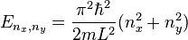
Since  and
and  can be interchanged without changing the energy, each energy level is at least twice as degenerate when and are different. Degenerate states are also obtained when the sum of squares of quantum numbers corresponding to different energy levels are the same.
and can be interchanged without changing the energy, each energy level is at least twice as degenerate when and are different. Degenerate states are also obtained when the sum of squares of quantum numbers corresponding to different energy levels are the same.
Due to the restrictions of the electronic states , quantum dots exhibit interesting finite size effects which dominate much of the physics involved with them. The most noticable of these finite size effects are in fluorescence, where quantum dots in the form of nanoparticles fluoresce at specific frequencies depending on the size of the nanoparticles.
Quantum dots do not have to be nanoparticles. Wecan create quantum dots by engineering quantum degnerate states of electrons in Single Walled Nanotubes (SWNTs) of Carbon or Boron Nitride:
Nanotube quantum dots have the advantage of the ease of being bridged from source to drain and being gated along the region where the degeneracy has been induced, via strain engineering or doping of the nanotube itself.
In the case of Carbon Nanotubes, esearchers need to be able to modify the electronic structure of the tubes so that different functionalities can be incorporated into the source-drain and gate electrode materials. This is difficult to do with pristine tubes because the sidewalls in these structures are extremely stable, which makes them difficult to chemically dope.
Scientists can produced arrays of quantum dots inside single-walled carbon nanotubes by producing a misalignment between the tube and an underlying silver substrate. The good thing about the technique is that it does not require any physical or chemical treatment on the tubes.
The electronic properties of carbon nanotubes are strongly influenced by the way the tubes are registered on metal substrates. Quantum confinements in the form of periodic quantum-well (QW) structures are produced over the whole length of the nanotube and the size of the confined regions can be controlled by changing the mismatch between the tube and substrate.
The band-structure of the nanotubes can also be manipulated depending on the degree of mismatch between the nanotube and substrate so that is resembles a superlattice in which the bandgap energy is periodically modulated. In turn, this produces periodic modulations of the nanotube's electronic structure, which then appears as 1D multiple quantum dots.
Thanks to the extremely small size of the confined region, the energy level splittings observed for the nanotubes are very large (around 260 meV), which means that the structure could operate as a quantum-dot system at room temperature rather than just at ultra-low temperatures.
Meanwhile, using strain engineering in carbon nanotubes, the coupling of electron spin in carbon nanotube quantum dots with the nanotube’s nanomechanical vibrations can significantly affect the spin of an electron trapped on it. Moreover, in this way the electronic band structure of the carbon nanotube itself can be affected by the electron’s spin.
The transport of electrons through SWNT quantum dots is induced using a conventional source and a drain electrode, which can be biased by a certain voltage. Electrons enter and leave the quantum dot one by one. The average number of electrons in the dot can be controlled by a gate voltage which adjusts the electrochemical potential. Due to the electrons entering and leaving the dot one by one, in confined energy quanta, the bridged and gated quantum dot functions as a single electron transistor:
Low energy band structure of SWNTs with open boundaries.
The determination of the transport properties of a SWNT quantum dot as a function of the applied voltages is a very well suited tool to analyze the electronic structure of SWNTs.
At low bias voltages the current can be turned off and on by varying the gate voltage. This is a consequence of the already mentioned, changing the gate voltage, which allows the transport of charge only for certain values of the electrochemical potential.
Due to the band and spin degrees of freedom, each of the SWNT shells can carry four electrons, leading to a fourfold periodicity of the current as a function of the gate voltage. The magnitude of the current allows for conclusions concerning the structure of the ground states for a certain number of electrons in the dot.
At finite bias voltages, transport measurements serve as excitation spectroscopy, determining the energy levels but also the nature of the excited states. Because of the 1D nature of a SWNT in combination with the Coulomb interaction, the elementary excitations of the system can not be described as fermionic quasiparticles as for higher dimensional systems, but as bosons. We calculate the transport properties of SWNTs quantum dots by using the so called reduced density matrix (RDM) formalism.
The state of the total system is described by the density matrix. The time evolution of the quantum dot degrees of freedom is governed by a nonunitary master equation and determines amongst others the current through the system. Since the energy spectrum of SWNTs reveals many degenerate states, coherences, i.e. superpositions of different states, have to be taken into account explicitly.
![\includegraphics[width=1.0\textwidth]{mfp-0900.0}](http://www.physik.uni-regensburg.de/forschung/grifoni/media/singlewallcarbonnanotubes-Dateien/Fig2.jpg) |
![\includegraphics[width=1.0\textwidth]{mfp-0900.0}](http://www.physik.uni-regensburg.de/forschung/grifoni/media/singlewallcarbonnanotubes-Dateien/Fig3.jpg) |

Current as a function of the gate and bias voltage. We find the Coulomb blockade regime with vanishing current. Additionally we find excitation lines, where the current changes since new excited states become involved in transport.
Simulated charge stability diagrams (Coulomb diamonds) of a Capacitive Coupled system of 3 Quantum Dots.
The first figure is switched at a logic 01 (#1)
+of+a+quantum+dot.png)
The second is switched at a logic of 10 (#2)
+of+a+quantum+dot+2.png)
Diamond Nitrogen Vacancy (NV)- Center Quantum Computer
Diamond NV centers may not have the best specs compared with other qubits, however they offer 3 major advantages:
(1) They work at room temperature
(2) They have very long coherence times
(3) They can be linked via photons, extending the capability of creating transferable protected information states.
(3) They can be linked via photons, extending the capability of creating transferable protected information states.

Although they are have only half the performance characteristics (i.e. benchmarking) of the Kane quantum computer, which has currently the best specifications of all existing solid state qubits, the diamond quantum computer has the greatest potential as it does not require near-absolute zero temperatures to operate which gets rid of the hassle of cooling.
Even so, the Kane quantum computer uses existing, electronic based architecture to work, where as the Diamond quantum computer requires optics and electronics. This may be a hindrance or a blessing in disguise as it may be easier to incorporate quantum information processing and cryptography within the diamond quantum computer using telecom wavelengths. Since diamond quantum computers are relatively new it may be decades before there true potential is unlocked.
Topological Quantum Computer
We have seen how 'Standard' qubits have been implemented in diverse physical systems, Now, as of 2014 the new discovery of topological protected states in certain materials, known as topological insulators, have sparked interest in the development of topological qubits, which can be created using a pair of Majorana fermions and could potentially be used for decoherence-free quantum computing.
Majorana Fermions are quasiparticles, theoretically predicted to form as excitations in superconductors. Majorana Fermions are their own antiparticles, this becomes possible because the superconductor imposes electron hole symmetry on the quasiparticle excitations. This creates a symmetry which is similar to the concept of the Dirac Fermion except that the quantum states for creation and annihilation are identical under the same order exchange operations.
Majorana fermion bound states at zero energy are therefore an example of non-abelian anyons: interchanging them changes the state of the system in a way which depends only on the order in which exchange was performed.
The non-abelian statistics that Majorana bound states possess allows to use them as a building block for a topological quantum computer.

Due to the fact that non-abelian anyons are their own antiparticles (hence they are Majorana Fermions), they will annihilate one another non-locally as they braid through the circuit. Hence the topology can manipulate the qubits and select which ones will annihilate.
Topological quantum computing also offers the prospect of powerful quantum computers that are also naturally fault-tolerant. Topology is the study of the global properties and spatial relations unaffected by a continuous change in the size or shape of objects like figures or graphs. Although engineering of a fault-tolerant quantum computer is in principle possible, it requires thousands of extra quantum bits to do so.

This is where topological quantum computation is of interest
as it provides natural fault-tolerance, thereby circumventing the need for
demanding engineering approaches. The fault-tolerance comes directly from the
quantum physics of ‘strongly correlated two-dimensional many-body quantum
systems’ known as Topological phases. Put very simply, in this case quantum
information is stored and processed within quantum states that are sensitive
only to the global structure, i.e. topology of these systems. This means that
the quantum errors, which are local, cannot affect it. This creates a much simpler way, in theory, to create a qubit which has self error correction.

The advantage of these qubits is that the braiding the non-abelian anyons perform in the circuit are non local and thus free from incoherence. This eliminates the need for complicated quantum error correction circuitry.
Quantum systems with
this property are said to be in a ‘topological phase’, similar to the topological phase electrons see when they interact with the flux quantum in the Aharanov-Bohm Effect.

The real work therefore involves searching for the signatures of
topological phases in quantum materials. Many such materials have been discovered already, such as bismuth telluride and
Within the last year, a research team from the Kavli Institute of Nanoscience at Delft University of Technology in the Netherlands reported an experiment involving indium antimonide superconducting nanowires connected to a circuit with a gold contact at one end and a slice of superconductor at the other. When exposed to a moderately strong magnetic field the apparatus showed a peak electrical conductance at zero voltage that is consistent with the formation of a pair of Majorana bound states, one at either end of the region of the nanowire in contact with the superconductor.
Many Theoretical models for developing different circuits using topological insulators to generate a quantum computer chip have been proposed, including T-shaped junctions in a type of Topologically protected Majorana transistor.
As shown by L. Hormozi, G. Zikos, N.E. Bonesteel, and S. H. Simon in the paperTopological Quantum Compling, one can use the braiding properties of the Fibonacci anyons to construct both an arbitrary SU(2) gate and a CNOT gate .

These authors pursued a brute-force approach which has the merit to show the possibility of realizing such a topological quantum computation but at the price of embarking, usually, in a very large searching procedure.

In the paper Topological Quantum Hashing with Icosahedral Group (byM. Burrello, H. Hu, G. Mussardo andX. Wan) a very efficient algorithm to implement an arbitrary SU(2) gate with the Fibonacci anyons has been proposed. Such an algorithm relies on the group structure of the icosahedral group (the largest discrete sub-group of SU(2)) and is able to pin down the target matrix with high accuracy in less than a second on a single 3GHz CPU.
Since the target matrix can be a unitary matrix, which itself can be a part of a group, G, a function defined on G can have a given symmetry where f remains unchanged under all possible group operations. This opens up the interesting possibility of using a quantum computer to find out when a situation arises when f is invariant only under a proper subgroup of G, a subgroup normally hidden, H, in a problem known appropriately enough as the hidden subgroup problem.
The technique of using algorithms to find these hidden subgroups is something which can be done easily with a quantum computer and is very difficult, if not impossible, with classical computer algorithms. It turns out that for a lot of the problems that quantum computers can do better than classical computers, the most fundamental advantage is that quantum algorithms are better at solving problems that involve symmetries, and that determining the number of symmetries in a function is fundamentally equivalent to determining the periodicity of the function over a given range of integers, hence the basis of performing functional operations that satisfy convolution theorems, such as Fourier analysis and other transforms (Laplacian, Mellin, etc.) along with the quantum algorithms that use it (such as Shor's algorithm), can be reduced to finding hidden symmetries in these operations and reducing them to fast matrix multiplication algorithms that work in the NP-hard regime, which will be of enormous importance in the field of computational complexity theory and in solving long standing problems, such as clique network problems which are of importance to everything from computational chemistry and bioinformatics to weather prediction and computer heuristics.
Quantum Algorithms
Instead of getting a Turing machine to work along a classical data string manipulating the 0s and 1s according to some program, at each timestep our quantum computer will apply a unitary transformation to the state space T.
After some sequence of unitary transformations have been applied (which we think of as a “quantum algorithm”), we measure the system.
Suppose we just had one qubit and we applied a load of unitary transformations to it (just unitary 2-by-2 matrices). If we started off with some vector, say  , and ended up with another one, say
  , we really want to get back to basics and know if we’ve got a 0 or a 1. However, because this is quantum mechanics, it’s quite possibly a superposition of the two. “Measuring” the qubit in a state therefore means:
, and ended up with another one, say , we really want to get back to basics and know if we’ve got a 0 or a 1. However, because this is quantum mechanics, it’s quite possibly a superposition of the two. “Measuring” the qubit in a state therefore means:- we consider the operator which projects the qubit onto the subspace spanned by
,
- this has eigenvalues 0 and 1 with eigenspaces spanned by
- when we measure the system we cause it to collapse into one or the other eigenspace and the number we measure is 0 (with probability
) or 1 (with probability
),
- in order to ensure that all probabilities sum up to 1 (which they surely should!) we need to normalise our states to have norm 1, i.e.
.
Quantum computing uses unitary matrix operators acting on discrete state vectors.
Using a matrix computing environment, we can simulating quantum algorithms to determine what a quantum computer could potentially do.
With such simulations, classical computers have shown to simulate the well-known quantum algorithms. To be brief, there is Shor's algorithm for factoring large numbers, Grover's search algorithm which allows you to do a "needle in a haystack" sort of search, and as well as the Quantum Fourier Transform (QFT) using quantum bits or qubits. We will go through each of these along with another, different type of quantum computation procedure.
Grover’s algorithm
Grover's Algorithm is a search algorithm that can search databases faster than any classical algorithm, by effectively finding the quantum basis state of the database.
To do this first we encode our database into a vector space. Remember our data consists of strings of length n (identification numbers for the N=2n objects) and colours (black or white) for each object (yes I know they’re not colours, it’s a figure of speech).
Introduce basis vectors  for each identification number and
  ,
,  for the colours. Form the tensor product
  (state space) so that a general basis element is something like
for each identification number and , for the colours. Form the tensor product (state space) so that a general basis element is something like
Next, we need to do unitary transformations for the algorithm
Let U be the unitary operator

(writing  for an arbitrary identification number) and let
for an arbitrary identification number) and let\rangle")
where ") denotes the colour of object and the coefficient is for normalisation (we want all states to have norm one). Finally we define
denotes the colour of object and the coefficient is for normalisation (we want all states to have norm one). Finally we define
denotes the colour of object and the coefficient is for normalisation (we want all states to have norm one). Finally we define
The funny notation need another word of explanation:  means the operator sending a vector
  to
to  (which is just a rescaling of by the number
  ).
).
means the operator sending a vector to (which is just a rescaling of by the number ).
These (U and V) are the unitary transformations we’ll use in Grover’s algorithm.
Notice that they’re both reflections: U reflects in the hyperplane orthogonal to all white vectors and V acts as -1 on the hyperplane  orthogonal to and preserves the vector .
orthogonal to and preserves the vector .The algorithm
We apply the composite transformation  to and specifically look at what happens to the vector which we defined above as
 \rangle") .
.
to and specifically look at what happens to the vector which we defined above as . What is the operation ? It’s a composition of two reflections and hence it’s a rotation. To understand exactly what’s rotating where, let’s write
  for the projection of to the subspace spanned by black vectors (normalising to have norm 1) and restrict attention to the 2-dimensional subspace spanned by and the vector
  , corresponding to the unique white vector in our dataset (where
  is the identification number of the unique white object).
Now is a linear combination of and by construction, say
is a linear combination of and by construction, say
Moreover, we know that the coefficient of in is  , so
, so
in is , so=1/\sqrt{N}.")
The two reflections U and V preserve the 2-dimensional subspace spanned by and the vector . Indeed, reflecting using U gives
and the vector . Indeed, reflecting using U gives
and the using V (exercise, very clear when you draw the picture!) gives
|\xi'\rangle+\sin(\phi+2\phi)|mW\rangle")
In other words, VU is a rotation by  towards . If we rotate R times then the -component of
 ^R|\xi\rangle") is
is
towards . If we rotate R times then the -component of is\phi)")
and (remembering our discussion about measurement) the square of this quantity
\phi)")
 has an interpretation as the probability that we get the right identification number for the white object when we measure the identification number in this state (i.e. after rotation). When N is large
  is very small and we can pick R to make very close to 1. Indeed, when N is enormous, so that
  it’s clear that we need
  , i.e.
Note: we don’t want to do any more than this, or else we start rotating away from
We only had to do Grover’s algorithm about  times to the right answer with high probability, which is a big saving – if we quadruple the number of objects in the database then classically we quadruple computing time, but with Grover’s algorithm we only double it.
times to the right answer with high probability, which is a big saving – if we quadruple the number of objects in the database then classically we quadruple computing time, but with Grover’s algorithm we only double it.
Of course, we need to repeat the experiment many times to get a probability distribution and pick the identification number which seems to occur with a frequency
but we can do this a fixed number of times (independently of N) because the probability that we get the right answer is improving with N. All in all, we quadratically save computational effort and it’s all thanks to the use of purely formal quantum mechanics.
Of course, it’s not clear to me how you would really implement this algorithm (How would you start the quantum computer in the state ? How would you actually do the unitary transformations?) so we should really treat it as a mathematical abstraction until further notice. However, it’s a simple and surprising illustration of the power of quantum mechanics.
? How would you actually do the unitary transformations?) so we should really treat it as a mathematical abstraction until further notice. However, it’s a simple and surprising illustration of the power of quantum mechanics.Quantum Fourier Transform (QFT)
The Quantum Fourier Transform (QFT) uses normalized basis functions (unlike the classical Discrete Fourier Transform) to represent a discrete state vector.
The Classical fourier transform maps the vector
into the vector

The Quantum Fourier Transform does pretty much the same thing. However it acts on quantum states --quantum versions of the vectors we saw in the classical case.
Thus a quantum basis vector

Using this we can see that the arbitrary state
The Quantum Fourier Transform (QFT) on state  maps it to
  , where
maps it to , where
(i.e arbitrary states are related by a fourier transform)
which is nothing but the classical discrete Fourier transform of the amplitudes. So QFT of the basis state  leads to
leads to
However instead of the above definition, it is much more convenient to adopt the product representation of QFT, which is

where  represents the binary fraction
  .
.
represents the binary fraction .
That the two definitions are equivalent is evident from the following straight forward algebra.
We start with state


![=\frac{1}{2^{n/2}}\bigotimes_{l = 1}^n \left[\sum_{k_l = 0}^1 e^{2\pi ij k_l2^-l}|k_l\big\rangle \right]](http://ictwiki.iitk.ernet.in/wiki/images/math/b/b/c/bbc1fe2b4598b264327ed4a35066b9f6.png)
![=\frac{1}{2^{n/2}}\bigotimes_{l = 1}^n \left[|0\big\rangle+2^{2\pi ij2^-l}|1\big\rangle \right]](http://ictwiki.iitk.ernet.in/wiki/images/math/e/c/0/ec01219ecee9f92df9324735f6a7f319.png)

The product representation makes the task of designing a quantum circuit for QFT much easier. The circuit is as shown below

in fig.[1]
In the circuit diagram,  and
and  is the Hadamard gate.
and is the Hadamard gate.
A key thing to note here is that the Quantum Fourier Transform is Unitary and thus can be implemented via coherent physical processes i.e. qubits on a Quantum Computer. By lining up the qubits in the appropriate quantum circuit (just as one might line up classical logic gates) one is able to compute the Quantum Fourier Transform.
However, the Quantum Computer is only more efficient at computing Quantum Fourier Transforms and not Classical Fourier Transforms. Thus the Quantum Fourier Transform does not necessarily provide any direct speedups for classical problems that require a Fourier Transform.
In particular it can be shown that the problem of finding r: the least integer such that

where x and N have no common factors. is equivalent to the prime factorization problem.
Armed with the Quantum Fourier Transform and the equivalence of order finding and factoring, one can find a quantum algorithm for factoring an integer, known as Shor's Algorithm.
Shor's algorithm
The problem of integer factorization, as it stands is of profound practical importance. Determination of prime factors of large integers is intractably hard though verification is easy. Classically integer factorization is (suspected) NPhard. This asymmetry is the basis of many cryptographic algorithms and digital signatures, like RSA. Best known classical algorithm for prime factorization, the number field sieve, runs in time.
time.
time. Shor’s algorithm is designed to do this, but it can only run on a quantum computer due to the use of the Quantum Fourier Transform, QFT, described beforehand. Using the QFT, one can derive an algorithm that runs in
 time for factoring an integer. Similar algorithms such as the general number field sieve can achieve the same result on classical computers but will take much longer. The quantum version runs in polynomial time, whereas the classic can only manage sub-exponential. The quantum computer is used to simultaneously calculate every value of a function.
Peter Shor in 1994 gave a randomized polynomial time quantum algorithm for prime factorization.
The algorithm, as proposed by Shor, goes as follows. To factorize a composite integer N,
1. Pick a random number 
2. Compute gcd  , if gcd
  , we are done
, if gcd , we are done
3. Using order finding sub-routine, find period  of
of  mod
mod 
of mod
4. If is odd, back to step 1
is odd, back to step 1
5. If  , back to step 1
, back to step 1
6. gcd  is a non-trivial factor of .
The programming steps in Shor's Algorithm is summarized in the flowchart below:
is a non-trivial factor of .The programming steps in Shor's Algorithm is summarized in the flowchart below:

The significance of the above algorithm is that the problem of integer factorization has been reduced to the problem of order finding. We have a randomized polynomial time Turing-type reduction of factorization to order-finding. If some how, order-finding is accomplished in polynomial time, our problem is solved.
Another technique that will be required is quantum phase estimation. The algorithm requires two quantum registers. First register of  qubits, intialised to state
  ( is determined by the required performance) stores the t-bit approximation of the phase, while the second register stores
  . Hadamard is applied to first register followed by controlled-U ops on the second register, with
  raised to successive powers of 2. In the next stage, inverse QFT is applied on register 1. Finally first register is measured in the computational basis to get bit approximate value for
  . The steps have been enlisted below.
qubits, intialised to state ( is determined by the required performance) stores the t-bit approximation of the phase, while the second register stores . Hadamard is applied to first register followed by controlled-U ops on the second register, with raised to successive powers of 2. In the next stage, inverse QFT is applied on register 1. Finally first register is measured in the computational basis to get bit approximate value for . The steps have been enlisted below.
1.  : Initial State
: Initial State
2. : Create superposition
: Create superposition
3.  : Apply series of controlled-U raised to successive powers of 2
: Apply series of controlled-U raised to successive powers of 2
4. : After applying inverse Fourier transform
: After applying inverse Fourier transform
5.  : Measure first register to get bit approximate value of
: Measure first register to get bit approximate value of
Circuit for Phase Estimation is given in the diagram below:

The order finding algorithm makes use of phase estimation algorithm. The goal is to find out period of  . In order to achieve this, the operator
  is employed.
. In order to achieve this, the operator is employed. which is defined as,
is an eigenstate of

However the trouble is,
is unknown, so preparing is out of question. But, it can be shown [6] that starting from j1i and using  we can estimate
  accurately upto
  bits with probability
  . Hence following the phase estimation algorithm,the order finding algorithm goes as follows,
1.  : Initial State
: Initial State
2.  : Create Superposition
: Create Superposition
3.  : Apply
  which performs
: Apply which performs 
4.  : After applying inverse QFT
: After applying inverse QFT
5.  : Measurement of first register
: Measurement of first register
6.  : Using Continued fractions algorithm
: Using Continued fractions algorithm
In order to compute the sequence of controlled  operations required by the phase estimation algorithm, we perform the following,
operations required by the phase estimation algorithm, we perform the following,


This is equivalent to a Modular exponentiation, which can be done using the fast exponentiation algorithm.
So, Shor's algorithm, at first reduces the problem of integer factorization, to that of order finding and then solves the order finding problem in polynomial time with bounded error.
The archetype quantum register used for the implementation of Shor's Algorithm is an organic molecule consisting of five 19 F and two 13 C nuclei, i.e. a total of seven spin-1/2 nuclei withing a Nuclear Magnetic Resonance, NMR, Quantum Computer:

Quantum architecture like this can be said to have begun with Seth Lloyd's 1993 proposal for a molecular chain computer.
For modular exponentiation,  qubits (first register) were used. For encoding
  qubits (second register) were used. Multiplication by
  mod 15 reduced to addition of
  controlled by qubit 3. This can be implemented using two CNOT. Multiplication by
  mod 15 in a 4-bit register can be implemented by swapping bits 0 with 2 and 1 with 3. Each swap can be implemented using two CNOTs. Hadamard and Phase gates (for QFT) can be achieved by spin selective rotations.
qubits (first register) were used. For encoding qubits (second register) were used. Multiplication by mod 15 reduced to addition of controlled by qubit 3. This can be implemented using two CNOT. Multiplication by mod 15 in a 4-bit register can be implemented by swapping bits 0 with 2 and 1 with 3. Each swap can be implemented using two CNOTs. Hadamard and Phase gates (for QFT) can be achieved by spin selective rotations.
Populations of the spin states are measured for the random numbers less than the number being factorized:
 For
For 
− Qubit 1 & 2 are found to be in state and qubit 3 in state 
and qubit 3 in state
− So resulting state is either
 or
or 
indicating a periodicity of and
and  .
.
or indicating a periodicity of
and .
 For
For 
− Qubit 1 found to be in state and qubit 2 and 3, in state
and qubit 2 and 3, in state
− So resulting states are

indicating a periodicity of n = 2, and  .
.
.
Hence for the 2 random numbers measured simultaneously on the resister, 11 and 7, the number 15, a prime number, has been factorized into 2 prime numbers, namely 3 and 5.
A different type of quantum computation- Adiabatic quantum computing
Fast search algorithms and factoring large primes may have seemed like the biggest application of quantum computing in their beginning, however there is huge applications in the field of optimization algorithms which quantum computer models could do to change a lot of fields, from engineering to .
It turns out that the Adiabatic model of quantum computation is very good at solving optimization problems.
Think for example of trying to find the shortest path on a map from one city to another. If you wanted to do a brute-force search, you'd be trying every single possibility that existed. Another example is the knapsack problem, where you have a bunch of items but you can only carry a certain amount. What's the value of each item versus its weight where there are n objects with weights w_i and values v_i?
The goal is to maximize the value of the objects selected, respecting a limit W on the sum of the weights of the selected objects. The vectors give the indices of the objects in order of their selection. In principle any vector (i_0, ..., i_{k - 1}) with sum_{j = 0}^{k - 1} w_{i_j} <= W is k-promising, but in order to assure that each selection is considered only once, we will impose as well that the i_j are increasing. So, we are searching a graph with in total 2^n nodes (all subsets of n elements). This graph is a tree. All leafs are potential solutions.

Because this is an optimization problem, the notion of solution is not entirely adequate, backtracking is rather designed for decision problems, in which one should answer questions of the type "is there a feasible solution?" or "is there a feasible solution achieving a value of at least V?". If we would ask the latter question, we could output a selection of objects as soon as sum_{j = 0}^{k - 1} v_{i_j} >= V. In this case the extension of a solution might again be a solution.
Maybe you're NASA and you're building a rocket, and you're trying to figure out how much fuel to put on the rocket. But remember fuel adds weight, so what are the optimal fuel to payload ratios? Perhaps you are studying protein folding, and you need to fold in the minimum energy conformation so that you can understand how diseases work (but nature doesn't always get to the minimum energy conformation, e.g. mad cow disease, sickle cell anemia). These are all massive problems with tons of simulated parameters.
Adiabatic quantum computing gives us a way to do these problems potentially much faster than classical computers. The trick lies in quantum tunneling. This figure makes that idea most obvious:

Imagine the black function as a hill. In our classical world, there is no way to get from one minima to another without walking over the hill. This is what all classical solver techniques must do, whether it's simple hill-climbing, simulated annealing, or genetic algorithms. Quantum annealers, however, can tunnel through sufficiently thin barriers (depending on the tunneling amplitude of the particle). You can intuitively see how much work it would take to go up that hill, and why it's not probable that any solver will know to do that, especially if it has no knowledge that the global minima is right over the edge. But it's effortless for the quantum particle, so this is helpful.
Briefly, ere is a small list of problems and application areas that could potentially be solved much more quickly with an AQC:
- Protein folding
- Shortest paths on a map
- Manufacturing and logistics
- Machine learning and AI
- Containment problem in nuclear fusion (materials simulation)
- Traffic engineering
- Computer vision (e.g. anomaly detection)
- Search ranking
- Image/video/data compression
- Scheduling of any sort (airline, events, computer process, etc.)
- Automatic theorem provers
And of course there are things that if we are able to do, like linear algebra, that will increase any real list like this by many, many times.
These problems, such as the knapsack type problems and others involving trees, can be reduced to the Boolean satisfiability problem, or SAT. Basically, it's an algebraic or Boolean expression that looks like ( ^ means AND, v means OR,
 means NOT):
As an example of this construction, if we have
= (x1

(
Because the only propositional connectives contained in the formula are and, or, and not, we say that this is a SAT that is in Conjunctive normal form, CNF. Since it contains 3 nodes, we call this a 3-CNF-SAT.
Letting = C1 C2 . . . Ck be a boolean formula in 3-CNF with k clauses. For r = 1, 2, . . . , k, each clause Cr has exactly three distinct literals . We shall construct a graph G such that is satisfiable if and only if G has a clique of size k. we can rewrite the formula to
= C1 C2 C3
where C1 = (x1 x2 x3), C2 =(x1 x2 x3), and C3 = (x1 x2 x3)
It is possible to convert the clique problem into algebraic form if you like, so that ANDs are the multiplication (*), ORs are addition (+), negation could be negative (-), etc. Then you have an algebraic expression. You can take that expression and represent it in summation form. A satisfying assignment of the formula is x1 = 0, x2 = 0, x3 = 1. This satisfying assignment satisfies C1 with x2, and it satisfies C2 and C3 with x3.
The graph G derived from the 3-CNF formula is

Graphs like the above are called clique networks, with the values corresponding to the clique having shaded vertices in the graph above. A clique in an undirected graph G = (V, E) is a subset V' V of vertices, each pair of which is connected by an edge in E. In other words, a clique is a complete subgraph of G. The size of a clique is the number of vertices it contains. The clique problem is the optimization problem of finding a clique of maximum size in a graph.
D-wave's Adiabatic Quantum Computer is primarily used to solve the Boolean satisfiability problem, like the clique problem, using the adiabatic Hamiltonian, where the solutions are the maxima and minima in terms of a graph where there is a collection of nodes in a grid. This graph is analogous to the "program" in an AQC, where the initial state of qubits are connected in a certain way.

Mapping a problem to a basic Boolean satisfiability problem can difficult or can create added work (imagine a problem that requires the number of qubits to scale with the number of real variables by a polynomial of high degree, or worse, exponentially). You might also find that an approximate solver is not good when you have hard constraints that must not be violated (these machines operate at finite temperature, so there is always noise). So the types of problems that can be solved are by no means universal.One thing that is easy for the Adiabatic Quantum Computer is quantum error correction. The adiabatic theorem tells you that the longer you wait for your system to reach its final state, the more likely you are to have stayed in the ground state (or, said another way, the less likely you are to have excitations, which basically translate to errors). Therefore, in order to reduce error, all you need to do is run the algorithm in the adiabatic quantum computer for a longer time. If you ran it for T = infinity, you'd be 100% accurate.
In terms of practicality, D-Wave has already built a 128-qubit AQC (as of early 2014, Google/NASA Ames share a 512-qubit machine), so on that front we are good. They're still trying to improve accuracy and such things, but their main goal is to get good answers within some tolerable tolerance. They've got big customers (Lockheed Martin, Google) wanting a piece of this, and they're looking like they're making a lot of progress. It is indeed a very exciting area of research to follow.
References
Richard Feynman (1982). "Simulating physics with computers". International Journal of Theoretical Physics 21 (6–7): 467
Gershenfeld & Chuang. Bulk Spin-Resonance Quantum Computation. Science, 275, 1997.
Nielsen & Chuang. Quantum Computation & Quantum Information Theory. Cam- bridge Univ. Press.
Vandersypen & Chuang. NMR techniques for quantum control and computation. RMP, 76, 2004.
Chuang et al. Experimental realization of Shor's quantum factoring algorithm using nuclear magnetic resonance. Nature, 414, 2001.
Nakahara & Ohmi. Quantum Computing. CRC Press.
Peter W. Shor. Polynomial-Time Algorithms for Prime Factorization and Discrete Logarithms on a Quantum Computer. arXiv:quant-ph, 1996
Aharonov, D., Ben-Or, M. Fault-tolerant quantum computation with constant error rate. In Proceedings of the Twenty-Ninth Annual ACM Symposium on Theory of Computing (1997). ACM, 176–188.
Aharonov, Y., Davidovich, L., Zagury, N. Quantum random walks. Phys. Rev. A 48, 167 (1993).
Ambainis, A. Quantum walk algorithm for element distinctness. SIAM J. Comput. 37 (2007), 210.
Ambainis, A., Kempe, J., Rivosh, A. Coins make quantum walks faster. In Proceedings of the 16th Annual ACM SIAM Symposium on Discrete Algorithms (2005), 1099.
Aspuru-Guzik, A., Dutoi, A., Love, P.J., head-Gordon, M. Simulated quantum computation of molecular energies. Science 309, 5741 (2005).
Bell, J.S. On the Einstein Podolsky Rosen paradox. Physics 1, (1964), 195.
Buhrman, H. Špalek, R. Quantum verification of matrix products. In Proceedings of the 17th Annual ACM-SIAM Symposium on Discrete Algorithms (2006), 880.
Childs, A.M., Cleve, R., Deotto, E., Farhi, E., Gutmann, S., Spielman, D.A. Exponential algorithmic speedup by quantum walk. In Proceedings of the 35th ACM Symposium on Theory of Computing (2003), 59–68.
Farhi, E., Gutmann, S. Quantum computation and decision trees. Phys. Rev. A 58 (1998), 915.
Farhi, E., Goldstone, J., Gutmann, S. A quantum algorithm for the Hamiltonian NAND tree. Eprint arXiv:quant-ph/0702144, 2007.
Feynman, R. Simulating physics with computers. Intl. J. Theor. Phys. 21 (1982), 467–488.
Grover, L. A fast quantum mechanical algorithm for database search. In Proceedings of the 28th Annual ACM Symposium on the Theory of Computation (New York, 1996). ACM, 212–219.
Häffner, H., Hänsel, W., Roos, C.F., Benhelm, J., al kar, D.C., Chwalla, M., Körber, T., Rapol, U.D., Riebe, M., Schmidt, P.O., Becher, C., Gühne, O., Dür, W., Blatt, R. Scalable multiparticle entanglement of trapped ions. Nature 438 (2005), 643.
Hallgren, S. Polynomial-time quantum algorithms for pell's equation and the principal ideal problem. InProceedings of the 34th Annual ACM Symposium on the Theory of Computation (New York, 2002). ACM, 653–658.
Kedlaya, K.S. Quantum computation of zeta functions of curves. Comput. Complex. 15, 1–19 (2006).
Kitaev, A. Quantum error correction with imperfect gates. In Quantum Communication, Computing and Measurement (New York, 1997). Plenum, 181–188.
Knill, E., Laflamme, R., Zurek, W.H. Resilent quantum computation. Science 279 (1998), 342–345.
Knill, E., Laflamme, R., Zurek, W.H. Resilient quantum computation: error models and thresholds. Proc. Roy. Soc. Lond. Ser. A 454 (1998), 365–384.
Leibfried, D., Knill, E., Seidelin, S., Britton, J., Blakestad, R.B., Chiaverini, J., Hume, D.B., Itano, W.M., Jost, J.D., Langer, C., Ozeri, R., Reichle, R., Wineland, D.J. Creation of a six-atom 'Schrödinger cat' state.Nature 438 (2005), 639.
Magniez, F., Santha, M., Szegedy, M. Quantum algorithms for the triangle problem. In Proceedings of the 16th Annual ACM SIAM Symposium on Discrete Algorithms (2005), 1109.
Nielsen, M.A. Chuang, I.L. Quantum Computation and Quantum Information. Cambridge University Press, New York, 2000.
Regev, O. Quantum computation and lattice problems. In 43rd Symposium on Foundations of Computer Science (IEEE Computer Society, 2002), 520–529.
Rivest, R.L., Shamir, A., Adleman, L. A method of obtaining digital signatures and public-key cryptosystems. Commun. ACM 21 (1978), 120–126.
Shor, P.W. Algorithms for quantum computation: Discrete log and factoring. In Proceedings of the 35th Annual Symposium on the Foundations of Computer Science. S. Goldwasser, ed. (Los Alamitos, CA, 1994). IEEE Computer Society, 124–134.
Shor, P.W. Fault tolerant quantum computation. In Proceedings of the 37th Symposium on the Foundations of Computer Science (Los Alamitos, CA, 1996), IEEE, 56–65.
Woehr, J. Online interview "A Conversation with Christos Papadimitriou". Dr. Dobb's J. July Dave Bacon is an assistant research professor in the Department of Computer Science and Engineering, Department of Physics, at the University of Washington, Seattle.
2. Beckman, D., Chari, A.N., Devabhaktuni, S. and Preskill, J. Efficient networks for quantum factoring. Phys. Rev. A 54 (1996), 1034–1063; http://arXiv.org/quant-ph/9602016.
3. Brown, K.L., Munro, W.J. and Kendon, V.M. Using quantum computers for quantum simulation. Entropy 12, 11 (2010), 2268–2307.
4. Buluta, I. and Nori, F. Quantum Simulators. Science 326, 5949 (2009), 108–111.
5. Childress, L. et al. Coherent dynamics of coupled electron and nuclear spin qubits in diamond. Science 314, 5797 (2006), 281–285.
6. Clark, C.R., Metodi, T.S., Gasster, S.D. and Brown, K.R. Resource requirements for fault tolerant quantum simulation: The ground state of the transverse Ising model. Phys. Rev. A 79, 6 (June 2009).
7. Devitt, S.J., Fowler, A.G., Stephens, A.M., Greentree, A.D., Hollenberg, L.C.L., Munro, W.J. and Nemoto, K. Architectural design for a topological cluster state quantum computer. New Journal of Physics 11 (2009).
8. Devitt, S.J., Fowler, A.G., Tilma, T., Munro, W.J. and Nemoto, K. Classical processing requirements for a topological quantum computing system. International Journal of Quantum Information 8 (2010), 1–27.
9. Devitt, S.J., Nemoto, K. and Munro, W.J. Quantum error correction for beginners. Reports on Progress in Physics 76, 8 (Aug. 2013).
10. DiVincenzo, D. The physical implementation of quantum computation. Fortschritte der Physik 48, 9-11 (2000), 771–783.
11. Fowler, A., Mariantoni, M., Martinis, J. and Cleland, A. A primer on surface codes: Developing a machine language for a quantum computer. Arxiv preprint (2012); arXiv:1208.0928.
12. Fowler, A.G., Devitt, S.J. and Hollenberg, L.C. Implementation of Shor's algorithm on a linear nearest neighbor qubit array. Quantum Information and Computation 4, 4 (2004), 237.
13. Gay, S. Quantum programming languages: Survey and bibliography. Bulletin of the European Association for Theoretical Computer Science (June 2005).
14. Isailovic, N., Whitney, M., Patel, Y. and Kubiatowicz, J. Running a quantum circuit at the speed of data. International Symposium on Computer Architecture. IEEE (2008), 177–188.
15. Jiang, L., Taylor, J.M., Sørensen, A.S. and Lukin, M.D. Distributed quantum computation based on small quantum registers. Phys. Rev. A 76 (Dec 2007).
16. Jones, N.C., Van Meter, R., Fowler, A.G., McMahon, P.L., Kim, J., Ladd, T.D. and Yamamoto, Y. Layered architecture for quantum computing. Phys. Rev. 2, 3 (July 2012), 031007.
17. Kielpinski, D., Monroe, C. and Wineland, D.J. Architecture for a large-scale ion-trap quantum computer. Nature 417 (2002), 709–711.
18. Kim, J. and Kim, C. Integrated optical approach to trapped ion quantum computation. Quantum Information and Computation 9, 2 (2009).
19. Ladd, T., Jelezko, F., Laflamme, R., Nakamura, Y., Monroe, C. and O'Brien, J. Quantum computers. Nature 464 (Mar. 2010), 45–53.
20. Lanyon, B.P. Universal digital quantum simulation with trapped ions. Science 334, 6052 (2011), 57–61.
21. Leibrandt, D. et al. Demonstration of a scalable, multiplexed ion trap for quantum information processing. Quantum Information and Computation 9, 901 (2009).
22. Levy, J.E. et al. Implications of electronics constraints for solid-state quantum error correction and quantum circuit failure probability. New Journal of Physics 13, 8 (2011).
23. Lloyd, S. A potentially realizable quantum computer. Science 261 (1993), 1569–1571.
24. Mariantoni, M. et al. Implementing the quantum von Neumann architecture with superconducting circuits. Science 334, 6052 (2011), 61–65.
25. Maslov, D., Falconer, S. and Mosca, M. Quantum Circuit Placement. IEEE Transactions on Computer-Aided Design of Integrated Circuits and Systems 27, 4 (2008), 752–763.
26. Metodi, T.S., Thaker, D.D., Cross, A.W., Chong, F.T. and Chuang, I.L. A quantum logic array microarchitecture: Scalable quantum data movement and computation. In Proceedings of the 2005 International Symposium on Microarchitecture (2005).
27. Monz, T. et al. 14-qubit entanglement: Creation and coherence. Phys. Rev. Lett 106, 13 (Mar. 2011).
28. Mosca, M. Quantum algorithms (2008); Arxiv preprint arXiv:0808.0369.
29. Oi, D.K.L., Devitt, S.J. and Hollenberg, L.C.L. Scalable error correction in distributed ion trap computers. Physical Review A 74, 052313 (2006).
30. Oskin, M., Chong, F.T., Chuang, I.L., and Kubiatowicz, J. Building quantum wires: The long and short of it. In Proceedings of the 30th Annual International Symposium on Computer Architecture (June 2003), ACM, N.Y.
31. Raussendorf, R., Harrington, J. and Goyal, K. Topological fault-tolerance in cluster state quantum computation. New Journal of Physics 9, 199 (2007).
32. Schindler, P., Barreiro, J.T., Monz, T., Nebendahl, V., Nigg, D., Chwalla, M., Hennrich, M. and Blatt, R. Experimental repetitive quantum error correction. Science 332, 6033 (2011), 1059–1061.
33. Shor, P.W. Algorithms for quantum computation: Discrete logarithms and factoring. In Proceedings of the 35th Symposium on Foundations of Computer Science. IEEE Computer Society Press, Los Alamitos, CA, 1994, 124–134.
34. Stace, T.M., Barrett, S.D. and Doherty, A.C. Thresholds for topological codes in the presence of loss. Physical Review Letters 102, 20 (2009).
35. Svore, K.M., Aho, A.V., Cross, A.W., Chuang, I. and Markov, I.L. A layered software architecture for quantum computing design tools. IEEE Computer (Jan 2006), 74–83.
36. Van Meter, R., Ladd, T.D., Fowler, A.G. and Yamamoto, Y. Distributed quantum computation architecture using semiconductor nanophotonics. International Journal of Quantum Information 8 (2010), 295–323.
37. Van Meter III, R.D. Architecture of a Quantum Multicomputer Optimized for Shor's Factoring Algorithm. Ph.D. thesis, Keio University, 2006; arXiv:quant-ph/0607065.
38. Vedral, V., Barenco, A. and Ekert, A. Quantum networks for elementary arithmetic operations. Phys. Rev. A 54 (1996), 147–153; http://arXiv.org/quant-ph/9511018.
39. Wootters, W.K. and Zurek, W.H. A single quantum cannot be cloned. Nature 299, 802 (Oct. 1982).
40. Yao, X.-C. et al. Experimental demonstration of topological error correction. Nature 482 (Feb. 2012), 489–494.
No comments:
Post a Comment
Note: only a member of this blog may post a comment.