
Abstract
Using a relatively simple custom "InfraBlue" filter and the imaging capabilities of the DJI Mavic Pro drone, I have been able to create Vegetation-Index maps with a surprising amount of resolution and detail considering the low-cost, ease of deployment and speed of the analysis of this procedure. It is hoped that this work can contribute to the already rich subject matter in this field, in particular the open-source communities involved with creating affordable and easy to use vegetation diagnostics for ecosystems, sustainable agriculture and environmental monitoring in general.
Introduction
Remote monitoring using photodetectors, ccd cameras etc. is a wide area of science and engineering. Ultimately it seeks to isolate key physical information from data obtained from detecting electromagnetic radiation, i.e. light. This physical information detected is all based on the interaction of light with matter.
The quantum theory of light tells us, in its simplest terms, that particles of light, photons, will excite electrons in atoms to a higher energy state and then be re-emitted by the electrons as they relax back to the ground state again. In a mixture of atoms, molecules, materials, and so forth we therefore expect a wide array, a broadband spectrum, of light photons at different wavelengths being absorbed, emitted and even transmitted directly through different forms of matter depending on the different excitation energies of the constituent atoms and molecules and the different transitions that can occur when light and matter interact.

EM Spectrum summarizing the ways light and matter interact.
The diagram above illustrates how EM radiation at different wavelengths interacts with matter in different degrees of excitation. at high energies, such as X-rays and extreme UV, EM radiation can break molecular bonds. EM in the near-UV to visible range typically electronically excites or fluoresces atoms and/or molecules. Infrared EM radiation however is usually only absorbed to induce molecular vibrations, causing no electronic transitions at all. As we get to longer wavelengths of EM radiation the more the radiation can travel through a material without being absorbed in a quantum mechanical action of an atom or molecule.
Electronic transitions in atoms are typically observed in the visible and ultraviolet regions, in the wavelength range approximately 200–700 nm. Near-infrared is a region of the electromagnetic spectrum (from 780 nm to 2500 nm) that offers particular interest for remote viewing.
Hyperspectral imaging is therefore a key diagnostic technology operating at wavelengths, including UV, Visible and, as we shall see in particular, Infrared Light. This ultimately allows monitoring of a landscape with which we want to get a full diagnostic of the nature of matter within, such as rocks, soils, plant life etc without much disturbance.
Near-infrared transitions in matter is based on molecular overtone and combination vibrations. electronic transitions using NIR are forbidden by the selection rules of quantum mechanics. A selection rule in quantum mechanics is merely the statement that an atom or a molecule, behaving as a harmonic oscillator may only absorb or emit a photon of light equal to the energy spacing between 2 energy levels. [Ref-1]
The basis for a spectroscopic selection rule is the value of the transition moment integral

where Ψ1 and Ψ2 are the wave functions of the two states involved in the transition and µ is the transition moment (probability) operator. If the value of this integral is zero the transition is forbidden.
In practice, the integral itself does not need to be calculated to determine a selection rule. It is sufficient to determine the symmetry of transition moment function. If the symmetry of this function spans the totally symmetric representation of the point group to which the atom or molecule belongs then its value is (in general) not zero and the transition is allowed. Otherwise, the transition is forbidden.
Electronic transitions may be forbidden using NIR, but vibrational transitions are allowed. in fact fundamental vibrational frequencies of a molecule corresponds to transition that do not behave like they do in the Harmonic Oscillator approximation. Molecules in bulk materials are then anharmonic oscillators, sometimes with some overlap between electronic and vibrational states but often the difference in electronic and vibrational energy levels is so great that they can be treated as separate transition hierarchies (so-called Born-Oppenheimer approximation).
So what does all of this mean for NIR sensing? As a main factor, the molar absorptivity in the near-IR region for materials can be typically quite small when compared to the rate at which materials absorb visible light. (also based on the Frank-Condon prinicple in which electronic transitions in matter will occur faster than vibronic transitions i.e. the movement of the atoms/molecules themselves) [Ref-2]
The advantage for use in remote viewing then is that NIR can typically penetrate much further into a sample than visible light and even much more than mid infrared radiation, (where overlap begins to happen between vibrational and rotational molecular energy levels). Near-infrared spectroscopy is, therefore, not a particularly sensitive technique, but it can be very useful in probing bulk material remotely.
For remote sensing in the environment there is yet another advantage to using NIR as the Sun itself emits very prominantly in the NIR, allowing for a greater molar absorbance deeper into bulk material which can then be detected as it is re-emitted by the bulk material. Hence even modestly sensitive cameras can be expected to detect a significant amount of this reflected radiation.

EM Spectrum summarizing the ways light and matter interact.
The diagram above illustrates how EM radiation at different wavelengths interacts with matter in different degrees of excitation. at high energies, such as X-rays and extreme UV, EM radiation can break molecular bonds. EM in the near-UV to visible range typically electronically excites or fluoresces atoms and/or molecules. Infrared EM radiation however is usually only absorbed to induce molecular vibrations, causing no electronic transitions at all. As we get to longer wavelengths of EM radiation the more the radiation can travel through a material without being absorbed in a quantum mechanical action of an atom or molecule.
Hyperspectral imaging is therefore a key diagnostic technology operating at wavelengths, including UV, Visible and, as we shall see in particular, Infrared Light. This ultimately allows monitoring of a landscape with which we want to get a full diagnostic of the nature of matter within, such as rocks, soils, plant life etc without much disturbance.
Near-infrared transitions in matter is based on molecular overtone and combination vibrations. electronic transitions using NIR are forbidden by the selection rules of quantum mechanics. A selection rule in quantum mechanics is merely the statement that an atom or a molecule, behaving as a harmonic oscillator may only absorb or emit a photon of light equal to the energy spacing between 2 energy levels. [Ref-1]
where Ψ1 and Ψ2 are the wave functions of the two states involved in the transition and µ is the transition moment (probability) operator. If the value of this integral is zero the transition is forbidden.
In practice, the integral itself does not need to be calculated to determine a selection rule. It is sufficient to determine the symmetry of transition moment function. If the symmetry of this function spans the totally symmetric representation of the point group to which the atom or molecule belongs then its value is (in general) not zero and the transition is allowed. Otherwise, the transition is forbidden.
NIR as a Plant Health Indicator
When studying the vegetation reflectance spectrum in detail, The near-infrared spectrum itself allows a relatively high detailed probe of the health of plants at a cellular level.
In photosynthesis, the chloroplasts in plant cells take absorb light energy sing chlorophyll which aborbs photons and creates and electronic channel to fix carbon and water to form glucose, the basis of carbohydrates and hence food for the plant.
The forms of chlorophyll in plants absorb light at specific frequencies, typically, in the red and blue light. The green portion of light is effectively reflected, this makes the plant was seen in the range of green in the visible spectrum.
This information is also important for developing lighting systems, for indoor agriculture for example, of which light frequencies are the most efficient for growing plants as exploited by so-called "grow lights" for indoor plant growth. This is another topic in precision agriculture which can be explored further.
In any case, Chlorophyll pigments A and B absorbs most energy at about 450 nm (blue) and 650 nm (red) respectively, with significant overlap between the 2 as shown in the diagram
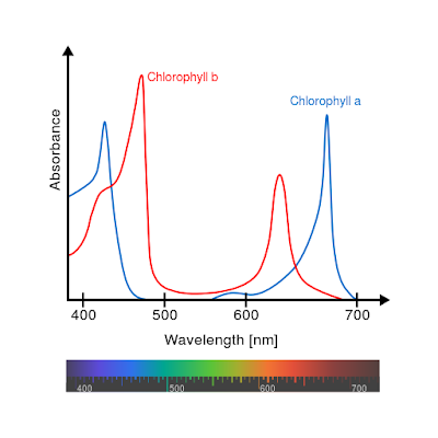
Other pigments absorb more visible wavelengths, but the most absorption occurs in the red and blue portions of the spectrum. This absorption removes these colors from the amount of light that is transmitted and reflected, causing the predominant visible color that reaches our eyes as green. This is the reason healthy vegetation appears as a dark green.
Unhealthy vegetation, on the other hand, will have less chlorophyll and thus will appear brighter (visibly) since less is absorbed and more is reflected to our eyes. This increase in red reflectance along with the green is what causes a general yellow appearance of unhealthy plants.
Plants reflect strongly in the NIR however not because of chlorophyll but because of a spongy layer of mesophyll tissue found on the bottom surface of the leaf, which does not reflect strongly in the red.
IR reflectance is advantageous to plants, as it is reflects electromagnetic energy that the plant cannot use and moreover would probably damage the plant tissues, especially during high levels of sunshine where the IR radiation would heat the plant tissues and slow down or damage cellular processes.
Plant stress causes an increase in visible light transmission in the green as the chlorophyll in the palisade mesophyll decays and the much more obvious effect of an increase in the reflectance of red.
The near-infrared plateau (NIR, 700 nm - 1100 nm), is a region where reflections are limited to the compounds typically found in the spongy mesophyll cells of leaves, made of primarily cellulose, lignin and other structural carbohydrates.
The spongy mesophyll cells located in the interior or back of the leaves reflects NIR light, much of which emerges as strong reflection rays. The intensity of NIR reflectance is commonly greater than most inorganic materials, so vegetation appears bright in NIR wavelengths.

NIR reflection in the Shortwave Infrared region is also affected by multiple scattering of photons within the leaf, related to the internal cellular structure, fraction of air spaces in the xylem vessels of the plant, and most important as a general indicator, the air-water interfaces that refract light within leaves.
The primary and secondary absorption of water in leaf reflectance are greatest in spectral bands centered at 1450, 1940, and 2500 nm, with important secondary absorptions at 980 nm, and 1240 nm [Ref-3]. These are the bands which create the primary NIR reflectance in healthy plants.
The spongy mesophyll tissue itself in plant foliage is critical for gas exchange, CO2 for use in photosynthesis and O2 for excretion as a waste product from the photosynthesis process itself. spongy mesophyll contains air gaps to allow for the gas exchange and also contains much of the vascular tissue of the leaf (with the xylem vessel portion facing into the spongy mesophyll and the phloem tubes facing towards the palisade mesophyll (where most photosynthesis occurs)

The cohesion-adhesion model of water transport in vascular plant tissue describes how hydrogen bonding in water to explain many key components of fluid movement through the plant's xylem and other vessels.
Within a vessel, water molecules hydrogen bond not only to each other, but also to the cellulose chain itself which comprises the wall of plant cells. This creates a capillary tube which allows for capillary action to occur since the vessel is relatively small. This mechanism allows plants to pull water up into their roots. Furthermore,hydrogen bonding can create a long chain of water molecules which can overcome the force of gravity and travel up to the high altitudes of leaves.

Cohesion-adhesion model of water transport in cellulose-based plant vascular tissue
Therefore the existing interface between the water in plants and the cellulose chains is a key indicator that a plant is #1 not under dehydration and #2 has structural integrity. If any one of these factors are removed, this indicates poor plant health and this is detected by the reflectance in the NIR.
Whenever a plant becomes either dehydrated or sickly, the spongy mesophyll layer collapses and this will cause the plant to reflect as less NIR light. Furthermore it will interrupt gas exchange thus causing the chloroplast containing palisade cells to die and cause the leaf to become more red.
Soil, on the other hand, reflects both NIR and Red .
Thus, a combination (approximated as linear) of the NIR reflectivity and red reflectivity should provide excellent contrast between plants and soil and between healthy plants and sick plants.
The Normalized Difference Vegetation Index (NDVI) is a simple graphical indicator that can be used to analyze remote sensing measurements, such as in aerial and space based surveys, and assess whether the target being observed contains live green vegetation or not.
It turns out which combination is not particularly important, but the NDVI index of (NIR-red)/(NIR+red) does happen to be particularly effective at normalizing for different irradiation conditions.
Hence, plants in a given area that are adequately hydrated show high absorbance of NIR light in this absorbance band (and low reflectance), whereas those subject to drying shows greater reflectance in this band.
NASA scientist Dr. Compton Tucker examined 18 different combinations of NIR (Landsat MSS 7 800-1100 nm), red (Landsat MSS 5 600-700 nm), and green (Landsat MSS 4 500-600 nm) and compared these results with the density of both wet and dry biomass to in an attempt determine which combination correlated best [Ref-4].
His findings were that
NIR/red,
SQRT(NIR/red),
NIR-red,
(NIR-red)/(NIR+red),
SQRT((NIR-red)/(NIR+red)+0.5)
all of the above are very similar indicators for estimating the density of photosynthetically active biomass, others go further in specific analysis using indices based the slopes of the line going across certain edges found in scatter plots of the NDVI vs RED pixels themselves. Others use forms of linear regression, support vector machines and trained neural networks to examine the hyperspectral images to look for patterns.
Typically one can use an experimentally determined threshold level for near IR reflectance from healthy plants to allow for a way to label plant health remotely.
When studying the vegetation reflectance spectrum in detail, The near-infrared spectrum itself allows a relatively high detailed probe of the health of plants at a cellular level.
In photosynthesis, the chloroplasts in plant cells take absorb light energy sing chlorophyll which aborbs photons and creates and electronic channel to fix carbon and water to form glucose, the basis of carbohydrates and hence food for the plant.
The forms of chlorophyll in plants absorb light at specific frequencies, typically, in the red and blue light. The green portion of light is effectively reflected, this makes the plant was seen in the range of green in the visible spectrum.
This information is also important for developing lighting systems, for indoor agriculture for example, of which light frequencies are the most efficient for growing plants as exploited by so-called "grow lights" for indoor plant growth. This is another topic in precision agriculture which can be explored further.
In any case, Chlorophyll pigments A and B absorbs most energy at about 450 nm (blue) and 650 nm (red) respectively, with significant overlap between the 2 as shown in the diagram
Other pigments absorb more visible wavelengths, but the most absorption occurs in the red and blue portions of the spectrum. This absorption removes these colors from the amount of light that is transmitted and reflected, causing the predominant visible color that reaches our eyes as green. This is the reason healthy vegetation appears as a dark green.
Unhealthy vegetation, on the other hand, will have less chlorophyll and thus will appear brighter (visibly) since less is absorbed and more is reflected to our eyes. This increase in red reflectance along with the green is what causes a general yellow appearance of unhealthy plants.
Plants reflect strongly in the NIR however not because of chlorophyll but because of a spongy layer of mesophyll tissue found on the bottom surface of the leaf, which does not reflect strongly in the red.
IR reflectance is advantageous to plants, as it is reflects electromagnetic energy that the plant cannot use and moreover would probably damage the plant tissues, especially during high levels of sunshine where the IR radiation would heat the plant tissues and slow down or damage cellular processes.
Plant stress causes an increase in visible light transmission in the green as the chlorophyll in the palisade mesophyll decays and the much more obvious effect of an increase in the reflectance of red.
The near-infrared plateau (NIR, 700 nm - 1100 nm), is a region where reflections are limited to the compounds typically found in the spongy mesophyll cells of leaves, made of primarily cellulose, lignin and other structural carbohydrates.
The spongy mesophyll cells located in the interior or back of the leaves reflects NIR light, much of which emerges as strong reflection rays. The intensity of NIR reflectance is commonly greater than most inorganic materials, so vegetation appears bright in NIR wavelengths.

NIR reflection in the Shortwave Infrared region is also affected by multiple scattering of photons within the leaf, related to the internal cellular structure, fraction of air spaces in the xylem vessels of the plant, and most important as a general indicator, the air-water interfaces that refract light within leaves.
The primary and secondary absorption of water in leaf reflectance are greatest in spectral bands centered at 1450, 1940, and 2500 nm, with important secondary absorptions at 980 nm, and 1240 nm [Ref-3]. These are the bands which create the primary NIR reflectance in healthy plants.
The spongy mesophyll tissue itself in plant foliage is critical for gas exchange, CO2 for use in photosynthesis and O2 for excretion as a waste product from the photosynthesis process itself. spongy mesophyll contains air gaps to allow for the gas exchange and also contains much of the vascular tissue of the leaf (with the xylem vessel portion facing into the spongy mesophyll and the phloem tubes facing towards the palisade mesophyll (where most photosynthesis occurs)

The cohesion-adhesion model of water transport in vascular plant tissue describes how hydrogen bonding in water to explain many key components of fluid movement through the plant's xylem and other vessels.
Within a vessel, water molecules hydrogen bond not only to each other, but also to the cellulose chain itself which comprises the wall of plant cells. This creates a capillary tube which allows for capillary action to occur since the vessel is relatively small. This mechanism allows plants to pull water up into their roots. Furthermore,hydrogen bonding can create a long chain of water molecules which can overcome the force of gravity and travel up to the high altitudes of leaves.

Cohesion-adhesion model of water transport in cellulose-based plant vascular tissue
Therefore the existing interface between the water in plants and the cellulose chains is a key indicator that a plant is #1 not under dehydration and #2 has structural integrity. If any one of these factors are removed, this indicates poor plant health and this is detected by the reflectance in the NIR.
Whenever a plant becomes either dehydrated or sickly, the spongy mesophyll layer collapses and this will cause the plant to reflect as less NIR light. Furthermore it will interrupt gas exchange thus causing the chloroplast containing palisade cells to die and cause the leaf to become more red.
Soil, on the other hand, reflects both NIR and Red .
Thus, a combination (approximated as linear) of the NIR reflectivity and red reflectivity should provide excellent contrast between plants and soil and between healthy plants and sick plants.
The Normalized Difference Vegetation Index (NDVI) is a simple graphical indicator that can be used to analyze remote sensing measurements, such as in aerial and space based surveys, and assess whether the target being observed contains live green vegetation or not.
It turns out which combination is not particularly important, but the NDVI index of (NIR-red)/(NIR+red) does happen to be particularly effective at normalizing for different irradiation conditions.
Hence, plants in a given area that are adequately hydrated show high absorbance of NIR light in this absorbance band (and low reflectance), whereas those subject to drying shows greater reflectance in this band.
His findings were that
NIR/red,
SQRT(NIR/red),
NIR-red,
(NIR-red)/(NIR+red),
SQRT((NIR-red)/(NIR+red)+0.5)
all of the above are very similar indicators for estimating the density of photosynthetically active biomass, others go further in specific analysis using indices based the slopes of the line going across certain edges found in scatter plots of the NDVI vs RED pixels themselves. Others use forms of linear regression, support vector machines and trained neural networks to examine the hyperspectral images to look for patterns.
Typically one can use an experimentally determined threshold level for near IR reflectance from healthy plants to allow for a way to label plant health remotely.
NDVI Imaging
NIR Image Sensing With Non-Specialized Cameras
Using a near-infrared spectral camera, a drone can easily monitor vegetation for signs of sickness and determine the health of both agricultural crops and the plants at the base of a foodchain in ecosystems to monitor an environment which is in a constant state of change.This is of utmost importance in parts of the world which are suffering from environmental destruction, both natural and increasingly induced by human activity. The surveillance of vegetation in endangered areas is of very high importance and new methods need to be introduced to ensure the survival of the most vulnerable biomes on earth, namely the tropical, temperate and boreal forests.
UAVs can also be used in crop monitoring and within what is called "precision agriculture", which works in order to optimize plantation management and assess more accurately the optimum density planting, in addition to making decisions regarding the use of fertilizers, irrigation frequency and other possibilities, such as to predict more accurately the crop production and allowing for sustainable use of the limited resources of water, soil and land available for agriculture.
The UAV can perform scheduled flights to carry out surveys of areas of vegetation (an indicated use, for example, for the of monitoring vulnerable ecosystems), and compare the spectral data taken from sensor cameras with available visual tomography, provided by accurate and updated maps, to detect and deduce root causes of detected instances of stress in the areas of plant growth.
However, with the sensor information itself we need to think a little more abstractly and find key variables which indicate the state of plant health, which is where NIR based imagining tools come in.
The traditional disadvantage of performing diagnostics on vegetation using NIR imaging is as follows:
- #1 Imaging of this kind is often expensive, often involving the use of hyperspectral cameras.
- #2 Suitable platforms, such as aircraft or satellites, are needed to allow for regular imaging to notice change in environments.
- #3 Technical expertise is needed to implement the survey programs themselves and to interpret image data in a meaningful way.
The growth of the commercial drone industry has solved issue #2. Commercial drone imaging is a true game-changer in the ease of deployment and how fast we can get image data - often in tandem with smartphones which allow for the use of phone-based applications to give meaningful diagnostics and perform actions based on them.

Problem #1 is beginning to be solved in some sense by commercial hyperspectral camera manufacturers. Hyperpectral cameras for use on drones have been coming down in price, moderately. However there is still a lot of expense involved, often more than the overhead costs of buying a drone itself.
For this reason there have been many projects that use the existing, monospectral cameras on drones to detect a portion of the near-infrared, using a filter that allows NIR to pass but filters one or more of the Red, Green or Blue bands so that we can assign the NIR band detected to one of these channels in a recorded image.
The filters I have made are a "Congo Blue" Lee filter combined with a UV filter to eliminate some fluorescence that the filter gel itself creates which can cause some over-saturation in the blue. I refer to this as an "Infrablue" filter.

As a first test, I used a smartphone camera under vibrant settings to detect the NIR reflectivity from a cactus. As you can see, NIR reflectivity is clearly assigned on the RED color channel on the camera sensor when equipped with the filter.
 NIR Through Smartphone Camera
Using my DJI Mavic Pro drone, I have, over the course of the summer and autumn of 2018, successfully deployed my filter on imaging flights in many different environments across Ireland and Cyprus - 2 countries with a wide range of different environmental conditions for vegetation to grow but nevertheless facing similar problems in different ways.
 My DJI Mavic Pro Drone (with pro platinum battery and propellers)
In 2018 Ireland experienced a relatively very dry summer, the driest in over 40 years under some estimates! This led to a perfect opportunity to compare with the normally arid conditions of Cyprus which, despite this, hosts a very abundant amount of vegetation across its rocky and arid landscape.
Using a near-infrared spectral camera, a drone can easily monitor vegetation for signs of sickness and determine the health of both agricultural crops and the plants at the base of a foodchain in ecosystems to monitor an environment which is in a constant state of change.This is of utmost importance in parts of the world which are suffering from environmental destruction, both natural and increasingly induced by human activity. The surveillance of vegetation in endangered areas is of very high importance and new methods need to be introduced to ensure the survival of the most vulnerable biomes on earth, namely the tropical, temperate and boreal forests.
UAVs can also be used in crop monitoring and within what is called "precision agriculture", which works in order to optimize plantation management and assess more accurately the optimum density planting, in addition to making decisions regarding the use of fertilizers, irrigation frequency and other possibilities, such as to predict more accurately the crop production and allowing for sustainable use of the limited resources of water, soil and land available for agriculture.
The UAV can perform scheduled flights to carry out surveys of areas of vegetation (an indicated use, for example, for the of monitoring vulnerable ecosystems), and compare the spectral data taken from sensor cameras with available visual tomography, provided by accurate and updated maps, to detect and deduce root causes of detected instances of stress in the areas of plant growth.
However, with the sensor information itself we need to think a little more abstractly and find key variables which indicate the state of plant health, which is where NIR based imagining tools come in.
The traditional disadvantage of performing diagnostics on vegetation using NIR imaging is as follows:
- #1 Imaging of this kind is often expensive, often involving the use of hyperspectral cameras.
- #2 Suitable platforms, such as aircraft or satellites, are needed to allow for regular imaging to notice change in environments.
- #3 Technical expertise is needed to implement the survey programs themselves and to interpret image data in a meaningful way.
The growth of the commercial drone industry has solved issue #2. Commercial drone imaging is a true game-changer in the ease of deployment and how fast we can get image data - often in tandem with smartphones which allow for the use of phone-based applications to give meaningful diagnostics and perform actions based on them.
Problem #1 is beginning to be solved in some sense by commercial hyperspectral camera manufacturers. Hyperpectral cameras for use on drones have been coming down in price, moderately. However there is still a lot of expense involved, often more than the overhead costs of buying a drone itself.
For this reason there have been many projects that use the existing, monospectral cameras on drones to detect a portion of the near-infrared, using a filter that allows NIR to pass but filters one or more of the Red, Green or Blue bands so that we can assign the NIR band detected to one of these channels in a recorded image.
The filters I have made are a "Congo Blue" Lee filter combined with a UV filter to eliminate some fluorescence that the filter gel itself creates which can cause some over-saturation in the blue. I refer to this as an "Infrablue" filter.

As a first test, I used a smartphone camera under vibrant settings to detect the NIR reflectivity from a cactus. As you can see, NIR reflectivity is clearly assigned on the RED color channel on the camera sensor when equipped with the filter.

NIR Through Smartphone Camera
Using my DJI Mavic Pro drone, I have, over the course of the summer and autumn of 2018, successfully deployed my filter on imaging flights in many different environments across Ireland and Cyprus - 2 countries with a wide range of different environmental conditions for vegetation to grow but nevertheless facing similar problems in different ways.

My DJI Mavic Pro Drone (with pro platinum battery and propellers)
In 2018 Ireland experienced a relatively very dry summer, the driest in over 40 years under some estimates! This led to a perfect opportunity to compare with the normally arid conditions of Cyprus which, despite this, hosts a very abundant amount of vegetation across its rocky and arid landscape.
Flight Test of Filter on Mavic Pro:
Most cameras, say on smart phones, use single-chip, either CMOS or CCD, sensors which can store images in RAW format in addition to the JPEG format using compression.
Any camera sensor will be arranged in grid of pixels to measure how much light is hitting a certain position. Most CMOS or CCD elements in cameras by themselves only measure a grey scale image, that is to say they only measure HSL (hue, saturation, lightness) and HSV (hue, saturation, value). There is no way to know, using a standard mono sensitive CCD or CMOS what proportion of red, green and blue light is measured from an image by themselves.
More expensive three and multi sensor cameras also exist, using separate sensors for the filtered red, green, blue color and beyond for true hyperspectral image capability and these can measure the relative proportion.
However the way single-chip cameras store RGB images is using a color filter array (CFA) to form a mosaic of the RGB detected. The most commonly used CFA is the Bayer mosaic filter array.
 Bayer Color Filter Array
The Bayer filter uses color filters and direct the individual colors red, green, blue onto individual pixels on the sensor, usually in an RGGB arrangement (i.e. 2X2 [RG;GB] ).
We have 2 greens per block because the human eye reacts more sensitively to green than to red or blue. We also detect brightness with much more intensity in the green band of the visible spectrum, so an image with more green elements should look sharper to the human eye.
With the DJI Mavic Pro I can capture 16 bit DNG photos, which means there are 16 bits (65,536) pixels and a pixel value range from 0 to 65,535 and standard JPEG images. When the camera saves a JPEG it compresses (removes) the pixels leaving a range of only 0 to 255. DNG format is just a fancy form of TIFF which contains RAW data values but with a lot more metadata such as linearisation information and color correction info which is needed for processing.
Due to the Bayer mosaic with 16 MP resolution therefore memory is allocated as 8 MP with red and blue (25% each) and 8 MP with green (50%) in an RGGB arrangement. We can read the data in a uint16 array in MATLAB
The RAW format does not necessarily store the colors in full resolution. It just means that the images are not compressed, as they would be in the case of JPEG images. Typically DNG files store uncompressed raw data from cameras in either color-corrected (using a color corrected matrix) RGB or Bayer RGB.
Using MATLAB, we can import and process the image in its original resolution, i.e. 4 MPs with red and blue, and 8 MPs in green.
How? By demosaicing the image, for instance using the MATLAB function demosaic. Demosaicing the image simply converts a Bayer pattern encoded image to a truecolor (RGB) image using a demosaicing algorithm of some kind.
Demosaicing (which is also called de-Bayering in our case) is used to reconstruct a full color image, with RGB values at every pixel, from the incomplete color samples output from an image sensor overlaid with a color filter array (CFA).

The JPEG format does this using a built in method in the camera. RAW format lets us control demosaicing ourselves. Several demosaicing methods exist, some use simple bilnear methods, others more complex. This is a wide area of engineering in and of itself and we shall only touch on a bit of it here.
In any effect this can interpolate the green pixels we remove from our image using the Infrablue filter : First, it define two gradients, one in horizontal direction, the other in vertical direction, for each blue/red position recorded.
Matlab has a demosaic function which can be set to use on an RGGB sensor alignment, turning into the original picture.
Here, as an exercise, I tried to implement a linear interpolation method for demosaicing myself by putting the mean of the same-color pixels around each unavailable pixel color, considering the bottom left and right top greens separately, because its neighbors change for each case across the image:

Pseudocode for Demosaicing (see Full Matlab Code Below)
I = imread('image.DNG');
[M,N,L] = size(I);
%Implement this as function J = demosaic(I) where I is an input mosaic image
%and T is an RGB output image.
J = zeros(M,N);
T = zeros(M,N,3);
figure,imshow(uint8(J));
%% Reconstruct Bayer Filtered Image here
for i = 2:M-1
for j = 2:N-1
if mod(i,2) == 0 && mod(j,2) == 1 %Green #1
T(i,j,1)=round((J(i-1,j)+J(i+1,j))/2);
T(i,j,2)=round(J(i,j));
T(i,j,3)=round((J(i,j-1)+J(i,j+1))/2);
elseif mod(i,2) == 1 && mod(j,2) == 0 Green #2
T(i,j,1)=round((J(i,j-1)+J(i,j+1))/2);
T(i,j,2)=round(J(i,j));
T(i,j,3)=round((J(i-1,j)+J(i+1,j))/2);
elseif mod(i,2) == 1 %Red
T(i,j,1)=round(J(i,j));
T(i,j,2)=round((J(i-1,j)+J(i+1,j)+J(i,j-1)+J(i,j+1))/4);
T(i,j,3)=round((J(i-1,j-1)+J(i+1,j-1)+J(i+1,j-1)+J(i-1,j+1))/4);
else %Blue
T(i,j,1)=round((J(i-1,j-1)+J(i+1,j-1)+J(i+1,j-1)+J(i-1,j+1))/4);
T(i,j,2)=round((J(i-1,j)+J(i+1,j)+J(i,j-1)+J(i,j+1))/4);
T(i,j,3)=round(J(i,j));
end
end
end
This demosaic function in effect allows the true colour image to be closely reconstructed even with the Infrablue filter in the front of the camera, which eliminates a lot of our green. An interesting trick!
 Reconstructed RGB Image (taken with "Infrablue" Filter)
The Mavik Pro Camera with a Infrablue filter measures Red (660 nm) on the RAW Data and Infrared (850 nm) on the JPEG to calculate the NDVI.
So by taking a RAW + JPEG image using an Infrablue filter with ertain exposure conditions (described in the Appendix) we can get an approximate RBG channel and a NIR channel.
We can do this using our demosaic process on the RAW image to get our approximate true colour RGB with a defined colour filter allignment, assigning each pixel to a channel, ie. (:,:,1)=red, (:,:,2)=green, (:,:,3)=blue.
Using our compressed JPEG we can assign the red pixels here as our NIR channel, i.e. (:,:,1) = nir.
 NIR JPEG Image
Assuming Bayer mosaic sensor alignment I create separate mosaic components for each colour channel from the processed RAW image and the JPEG image i.e.
J4 = RAWimg(1:2:end, 1:2:end); % For the 'True colour' i.e VIS Channel
J1 = jpgData(2:2:end, 2:2:end); % For the Constructed NIR Channel
Diagram to illustrate:
It is now possible to make InfraBlue Index Calculations by assigning values to each colour channel and summing our index across each pixel.
VIS = im2single(J4(:,:,1)); %VIS Channel RED - which is the highest intensity NIR used as a magnitude scale
NIR = im2single(J1(:,:,1)); %NIR Channel RED which is the IR reflectance of healthy vegetation
IBndvi = (VIS - NIR)./(VIS + NIR); %This is my Infrablue Index - a sort of quasi-NDVI
IBndvi = double(IBndvi);
Using this technique on infra blue images obtained from different environments we can get a "temperature" map of sorts showing vegetation density. Taking advantage of the long and sunny summer we had in Ireland and a trip to Cyprus* I got many NIR images with the drone to analyse and compare.
 Environment #1 - Public Park (Ireland)
 Environment #2 - Moorland (Ireland)
 Environment #3 - Beach and Shoreline (Ireland)
 Environment #4 - Desert Beach (Karpaz Peninsula- Cyprus)
 Environment #5 - Mountain Slope (Cyprus)
 Environment #6 - Mountain Slope (Ireland)
Flight Test of Filter on Mavic Pro:
Most cameras, say on smart phones, use single-chip, either CMOS or CCD, sensors which can store images in RAW format in addition to the JPEG format using compression.
Any camera sensor will be arranged in grid of pixels to measure how much light is hitting a certain position. Most CMOS or CCD elements in cameras by themselves only measure a grey scale image, that is to say they only measure HSL (hue, saturation, lightness) and HSV (hue, saturation, value). There is no way to know, using a standard mono sensitive CCD or CMOS what proportion of red, green and blue light is measured from an image by themselves.
More expensive three and multi sensor cameras also exist, using separate sensors for the filtered red, green, blue color and beyond for true hyperspectral image capability and these can measure the relative proportion.
However the way single-chip cameras store RGB images is using a color filter array (CFA) to form a mosaic of the RGB detected. The most commonly used CFA is the Bayer mosaic filter array.

Bayer Color Filter Array
The Bayer filter uses color filters and direct the individual colors red, green, blue onto individual pixels on the sensor, usually in an RGGB arrangement (i.e. 2X2 [RG;GB] ).
We have 2 greens per block because the human eye reacts more sensitively to green than to red or blue. We also detect brightness with much more intensity in the green band of the visible spectrum, so an image with more green elements should look sharper to the human eye.
With the DJI Mavic Pro I can capture 16 bit DNG photos, which means there are 16 bits (65,536) pixels and a pixel value range from 0 to 65,535 and standard JPEG images. When the camera saves a JPEG it compresses (removes) the pixels leaving a range of only 0 to 255. DNG format is just a fancy form of TIFF which contains RAW data values but with a lot more metadata such as linearisation information and color correction info which is needed for processing.
Due to the Bayer mosaic with 16 MP resolution therefore memory is allocated as 8 MP with red and blue (25% each) and 8 MP with green (50%) in an RGGB arrangement. We can read the data in a uint16 array in MATLAB
The RAW format does not necessarily store the colors in full resolution. It just means that the images are not compressed, as they would be in the case of JPEG images. Typically DNG files store uncompressed raw data from cameras in either color-corrected (using a color corrected matrix) RGB or Bayer RGB.
Using MATLAB, we can import and process the image in its original resolution, i.e. 4 MPs with red and blue, and 8 MPs in green.
How? By demosaicing the image, for instance using the MATLAB function demosaic. Demosaicing the image simply converts a Bayer pattern encoded image to a truecolor (RGB) image using a demosaicing algorithm of some kind.
Demosaicing (which is also called de-Bayering in our case) is used to reconstruct a full color image, with RGB values at every pixel, from the incomplete color samples output from an image sensor overlaid with a color filter array (CFA).

The JPEG format does this using a built in method in the camera. RAW format lets us control demosaicing ourselves. Several demosaicing methods exist, some use simple bilnear methods, others more complex. This is a wide area of engineering in and of itself and we shall only touch on a bit of it here.
In any effect this can interpolate the green pixels we remove from our image using the Infrablue filter : First, it define two gradients, one in horizontal direction, the other in vertical direction, for each blue/red position recorded.
Matlab has a demosaic function which can be set to use on an RGGB sensor alignment, turning into the original picture.
Here, as an exercise, I tried to implement a linear interpolation method for demosaicing myself by putting the mean of the same-color pixels around each unavailable pixel color, considering the bottom left and right top greens separately, because its neighbors change for each case across the image:

Pseudocode for Demosaicing (see Full Matlab Code Below)
I = imread('image.DNG');
[M,N,L] = size(I);
%Implement this as function J = demosaic(I) where I is an input mosaic image
%and T is an RGB output image.
J = zeros(M,N);
T = zeros(M,N,3);
figure,imshow(uint8(J));
%% Reconstruct Bayer Filtered Image here
for i = 2:M-1
for j = 2:N-1
if mod(i,2) == 0 && mod(j,2) == 1 %Green #1
T(i,j,1)=round((J(i-1,j)+J(i+1,j))/2);
T(i,j,2)=round(J(i,j));
T(i,j,3)=round((J(i,j-1)+J(i,j+1))/2);
elseif mod(i,2) == 1 && mod(j,2) == 0 Green #2
T(i,j,1)=round((J(i,j-1)+J(i,j+1))/2);
T(i,j,2)=round(J(i,j));
T(i,j,3)=round((J(i-1,j)+J(i+1,j))/2);
elseif mod(i,2) == 1 %Red
T(i,j,1)=round(J(i,j));
T(i,j,2)=round((J(i-1,j)+J(i+1,j)+J(i,j-1)+J(i,j+1))/4);
T(i,j,3)=round((J(i-1,j-1)+J(i+1,j-1)+J(i+1,j-1)+J(i-1,j+1))/4);
else %Blue
T(i,j,1)=round((J(i-1,j-1)+J(i+1,j-1)+J(i+1,j-1)+J(i-1,j+1))/4);
T(i,j,2)=round((J(i-1,j)+J(i+1,j)+J(i,j-1)+J(i,j+1))/4);
T(i,j,3)=round(J(i,j));
end
end
end
This demosaic function in effect allows the true colour image to be closely reconstructed even with the Infrablue filter in the front of the camera, which eliminates a lot of our green. An interesting trick!
Reconstructed RGB Image (taken with "Infrablue" Filter)
The Mavik Pro Camera with a Infrablue filter measures Red (660 nm) on the RAW Data and Infrared (850 nm) on the JPEG to calculate the NDVI.
So by taking a RAW + JPEG image using an Infrablue filter with ertain exposure conditions (described in the Appendix) we can get an approximate RBG channel and a NIR channel.
We can do this using our demosaic process on the RAW image to get our approximate true colour RGB with a defined colour filter allignment, assigning each pixel to a channel, ie. (:,:,1)=red, (:,:,2)=green, (:,:,3)=blue.
Using our compressed JPEG we can assign the red pixels here as our NIR channel, i.e. (:,:,1) = nir.

NIR JPEG Image
Assuming Bayer mosaic sensor alignment I create separate mosaic components for each colour channel from the processed RAW image and the JPEG image i.e.
J4 = RAWimg(1:2:end, 1:2:end); % For the 'True colour' i.e VIS Channel
J1 = jpgData(2:2:end, 2:2:end); % For the Constructed NIR Channel
Diagram to illustrate:
It is now possible to make InfraBlue Index Calculations by assigning values to each colour channel and summing our index across each pixel.
VIS = im2single(J4(:,:,1)); %VIS Channel RED - which is the highest intensity NIR used as a magnitude scale
NIR = im2single(J1(:,:,1)); %NIR Channel RED which is the IR reflectance of healthy vegetation
IBndvi = (VIS - NIR)./(VIS + NIR); %This is my Infrablue Index - a sort of quasi-NDVI
IBndvi = double(IBndvi);
Using this technique on infra blue images obtained from different environments we can get a "temperature" map of sorts showing vegetation density. Taking advantage of the long and sunny summer we had in Ireland and a trip to Cyprus* I got many NIR images with the drone to analyse and compare.
Environment #1 - Public Park (Ireland)
Environment #2 - Moorland (Ireland)
Environment #3 - Beach and Shoreline (Ireland)
Environment #4 - Desert Beach (Karpaz Peninsula- Cyprus)
Environment #5 - Mountain Slope (Cyprus)
Environment #6 - Mountain Slope (Ireland)
In order to identify pixels most likely to contain significant vegetation, you can apply a simple threshold to the image.(For example a 70% threshold to the original Cyprus Mountainside Image)
 The advantage of this is that the color gradient has been simplified which is an important step if we want to perform more complex processing in the future, such as image segmentation.
We can also look for indicators in the pixel information itself, by plottting the NIR pixel data versus the VIS (i.e. Red Channel) data to profile the intermix of dry areas, such as a definitive soil line, with vegetation density.

To link the spectral and spatial content, I can locate above-threshold pixels on the NIR-red scatter plot, re-drawing the scatter plot with the above-threshold pixels in a contrasting color (green) and then re-displaying the threshold NDVI image using the same blue-green color scheme.
The pixels having an NDVI value above the threshold appear to the upper left of the rest and correspond to the redder pixels in the CIR composite displays.

Pixels falling in the red regions indicate the most dense vegetation, green pixels represent more sparse vegetation intermixed with soil but pixels near the edge represent a soil line indicating little to no present vegetation. All areas between indicate a mix of soil and vegetation.
By defining edges of these regions, we see the number of pixels that overlap between the near-infrared and red channels decrease at certain edges of the scatter plot, which makes sense only if there is little to no vegetation here, which would reflect nir radiation into the camera in this region.
We can look at the soil profiles of the mountainside data from Ireland (Env #5) and Cyprus (Env #6) and compare them.
 Ireland (mountainside)
 Cyprus (mountainside)
Interesting to note how there appears to be a central dry region in the photograph from Cyprus which is not seen in the pixel distribution from Ireland. The pixel information appears to form into two separate regions with 2 distinct dry edges, perhaps due to the mountain elevation creating different bands of vegetation density?
Future Work...
- Involving Analysis:
Work in the area of looking for specific indicators in the image data is ongoing. Further work on the software and analysis side of things can include image segmentation, which adds much more structure to our interpretation of such images beyond what we may simply interpret using comparative analysis alone.
Segmentation based on different ndvi thresholds across the image is a key way of delineating prominent structures in an input image for post processing such as texture based analysis, feature extraction, selection, and classification.
By combining heuristic based image segmentation with stochastic modeling we can develop meta-heuristic methods to identify ndvi intensity thresholds and develop the principle of classification of sections of the image based on the thresholds.
With metaheuristics we effectively marry a a probabilistic approach with an established threshold segmentation procedure to improve the partitioning of the initial segmented image obtained by the initial threshold segmentation technique.
The various metaheuristic methods come from broad areas of signalling theory applied to data sets, pixels in our case. The pixels are essentially clustered in locations for classification, Gaussian centroids for example in K-means clustering. We then need pick a meta-heuristic procedure which can form these clusters in local and global minima.
- Involving New Hardware:
The release of the new Mavic Version 2 Drones (The Mavic Pro 2 and Mavic Zoom) are of course the prime focus of any future developments in this field of easy to deploy drone-based vegetation evaluation with the cheap and easy to process filter technology I have showcased here.
Just at a cursory look of these new drones specifications I can say the pixel volume (20MP) on the Hasselbrad Camera on the Mavic Pro 2 may allow for provide extra color assignment channels, critical to create more broad scheme vegetation evaluation via the Mavic Pro 2 camera.
The Mavic Zoom meanwhile has the capability to actively focus in on a region of interest which, with some clever hands on photography experience, may allow the user to eliminate the reduction in sensitivity seen on the edges of the typical NIR images taken using the old Mavic Pro.
This is an experimental science so only by using these new drone models with the InfraBlue technology can we know for certain. This will be the focus (finances permitting!) of my own future work in this area as I will be interested in purchasing a new Mavic model in the near future and creating a new version of an Infrablue filter for it.
In order to identify pixels most likely to contain significant vegetation, you can apply a simple threshold to the image.(For example a 70% threshold to the original Cyprus Mountainside Image)
The advantage of this is that the color gradient has been simplified which is an important step if we want to perform more complex processing in the future, such as image segmentation.

We can also look for indicators in the pixel information itself, by plottting the NIR pixel data versus the VIS (i.e. Red Channel) data to profile the intermix of dry areas, such as a definitive soil line, with vegetation density.

The pixels having an NDVI value above the threshold appear to the upper left of the rest and correspond to the redder pixels in the CIR composite displays.

Pixels falling in the red regions indicate the most dense vegetation, green pixels represent more sparse vegetation intermixed with soil but pixels near the edge represent a soil line indicating little to no present vegetation. All areas between indicate a mix of soil and vegetation.
By defining edges of these regions, we see the number of pixels that overlap between the near-infrared and red channels decrease at certain edges of the scatter plot, which makes sense only if there is little to no vegetation here, which would reflect nir radiation into the camera in this region.
We can look at the soil profiles of the mountainside data from Ireland (Env #5) and Cyprus (Env #6) and compare them.

Ireland (mountainside)

Cyprus (mountainside)
Interesting to note how there appears to be a central dry region in the photograph from Cyprus which is not seen in the pixel distribution from Ireland. The pixel information appears to form into two separate regions with 2 distinct dry edges, perhaps due to the mountain elevation creating different bands of vegetation density?
Future Work...
- Involving Analysis:
Work in the area of looking for specific indicators in the image data is ongoing. Further work on the software and analysis side of things can include image segmentation, which adds much more structure to our interpretation of such images beyond what we may simply interpret using comparative analysis alone.
The various metaheuristic methods come from broad areas of signalling theory applied to data sets, pixels in our case. The pixels are essentially clustered in locations for classification, Gaussian centroids for example in K-means clustering. We then need pick a meta-heuristic procedure which can form these clusters in local and global minima.
- Involving New Hardware:
Just at a cursory look of these new drones specifications I can say the pixel volume (20MP) on the Hasselbrad Camera on the Mavic Pro 2 may allow for provide extra color assignment channels, critical to create more broad scheme vegetation evaluation via the Mavic Pro 2 camera.
The Mavic Zoom meanwhile has the capability to actively focus in on a region of interest which, with some clever hands on photography experience, may allow the user to eliminate the reduction in sensitivity seen on the edges of the typical NIR images taken using the old Mavic Pro.
This is an experimental science so only by using these new drone models with the InfraBlue technology can we know for certain. This will be the focus (finances permitting!) of my own future work in this area as I will be interested in purchasing a new Mavic model in the near future and creating a new version of an Infrablue filter for it.
*Thanks!
A big thanks to the Galkin Family for their great assistance in the acquisition of this data across Ireland and Cyprus. This research would not have been possible without their provision of transportation, navigation and expertise in regards to the flight of drones and their knowledge of the landscapes of interest for drone photography in Cyprus.
References:
[Ref-1] - [Practical Guide to Interpretive Near-Infrared Spectroscopy By Jerry Workman, Jr., Lois Weyer]
[Ref-2] - [IUPAC Compendium of Chemical Terminology, 2nd Edition (1997)]
[Ref-3] - Carter, G.A. (1991) Primary and Secondary Effects of Water Content on the Spectral Reflectance of Leaves. American Journal of Botany, 78, 916-924.
[Ref-4] - Dr. Compton J. Tucker “Red and Photograghic Infrared Linear Combinations for Monitoring Vegetation.” - NASA 1979
Appendix:
NDVI image capture settings for Mavic Pro
Please note that these settings are a suggestion - you may want to adjust settings for your environment, or experiment to achieve the best results.
In the DJI GO app, select the bottom right settings icon and adjust the camera settings.
The Infrablue filter blocks a large portion of the ambient and direct sunlight so apply approximately these settings in the daylight and at the area of interest for best results.
The best way to tune the camera settings is to launch the drone with the camera facing downwards and then tune the settings shown below such that you get a clear and balanced NDVI photo.
Camera Settings - Vibrant image
Output - HD RAW+JPEG
ISO: 100 (to reduce noise)
Shutter: (1/200 or faster)
The shutter speed should be increased if the image appears to be over exposed. The more exposure the better as the sensitivity to NIR is very low.
Experience shows that the center of the image will contain the clearest data while the edges may become blurred.
Matlab Demo Code for DNG File Demosaicing
The image processing workflow is as follows:
% Custom Matlab Code for Demosaicing
% J. Campbell 2018
%DNG is just a fancy form of TIFF. So we can read DNG with TIFF class in MATLAB
warning off MATLAB:tifflib:TIFFReadDirectory:libraryWarning
filename = 'DJI_0011.DNG'; % Put file name here
t = Tiff(filename,'r');
offsets = getTag(t,'SubIFD');
setSubDirectory(t,offsets(1));
raw = read(t);
%As a demo, display RAW image
figure(1);
imshow(raw);
close(t);
% We will need some of the metadata from the DNG file for processing later
meta_info = imfinfo(filename);
% Crop to only valid pixels
x_origin = meta_info.SubIFDs{1}.ActiveArea(2)+1; % +1 due to MATLAB indexing
width = meta_info.SubIFDs{1}.DefaultCropSize(1);
y_origin = meta_info.SubIFDs{1}.ActiveArea(1)+1;
height = meta_info.SubIFDs{1}.DefaultCropSize(2);
raw = double(raw(y_origin:y_origin+height-1,x_origin:x_origin+width-1));
J = raw;
[M,N,L] = size(J);
T = zeros(M,N,3);
%% Demosaicing Process to Construct RGB Pixel Image from Bayer Filtered Pixel Image
for i = 2:M-1
for j = 2:N-1
if mod(i,2) == 0 && mod(j,2) == 1 %Green
T(i,j,1)=round((J(i-1,j)+J(i+1,j))/2);
T(i,j,2)=round(J(i,j));
T(i,j,3)=round((J(i,j-1)+J(i,j+1))/2);
elseif mod(i,2) == 1 && mod(j,2) == 0
T(i,j,1)=round((J(i,j-1)+J(i,j+1))/2);
T(i,j,2)=round(J(i,j));
T(i,j,3)=round((J(i-1,j)+J(i+1,j))/2);
elseif mod(i,2) == 1 %Red
T(i,j,1)=round(J(i,j));
T(i,j,2)=round((J(i-1,j)+J(i+1,j)+J(i,j-1)+J(i,j+1))/4);
T(i,j,3)=round((J(i-1,j-1)+J(i+1,j-1)+J(i+1,j-1)+J(i-1,j+1))/4);
else %Blue
T(i,j,1)=round((J(i-1,j-1)+J(i+1,j-1)+J(i+1,j-1)+J(i-1,j+1))/4);
T(i,j,2)=round((J(i-1,j)+J(i+1,j)+J(i,j-1)+J(i,j+1))/4);
T(i,j,3)=round(J(i,j));
end
end
end
%%reconstruct image
%assign new color channels
r = T(:,:,1);
g = T(:,:,2);
b = T(:,:,3);
figure (2)
%rough demosaic
rgb = cat(3,r,g,b);
%linearised color demosaic
temp = uint16(rgb/max(rgb(:))*2^16);
lin_rgb = double(temp)/2^16;
imshow(lin_rgb);
%Color Space Correcting For True Color Image Output
% - - - Color Correction Matrix from DNG Info - - -
temp2 = meta_info.ColorMatrix2;
xyz2cam = reshape(temp2,3,3)';
% Define transformation matrix from sRGB space to XYZ space for later use
rgb2xyz = [0.4124564 0.3575761 0.1804375;
0.2126729 0.7151522 0.0721750;
0.0193339 0.1191920 0.9503041];
rgb2cam = xyz2cam * rgb2xyz; % Assuming previously defined matrices
rgb2cam = rgb2cam ./ repmat(sum(rgb2cam,2),1,3); % Normalize rows to 1
cam2rgb = rgb2cam^-1;
lin_srgb = apply_cmatrix(lin_rgb, cam2rgb);
lin_srgb = max(0,min(lin_srgb,1)); % Always keep image clipped b/w 0-1
%%Brightness and Contast Control
grayim = rgb2gray(lin_srgb);
grayscale = 0.25/mean(grayim(:));
bright_srgb = min(1,lin_srgb*grayscale);
%gamma correction power function
%nl_srgb = bright_srgb.^(1/2.2);
nl_srgb = imadjust(bright_srgb, [0.06, 0.94], [], 0.45); %Adjust image intensity, and use gamma value of 0.45
nl_srgb(:,:,2) = nl_srgb(:,:,2)*0.60; %Reduce the green channel by factor of 0.60
nl_srgb(:,:,3) = nl_srgb(:,:,3)*0.90; %Reduce the blue channel by factor of 0.90
%%Congratulations, you now have a color-corrected, displayable RGB image.
figure(3);
imshow(nl_srgb);