The Path Integral Interpretation of Quantum Mechanics

The Path-integral Interpretation of Quantum Mechanics is a rigorous formulation of quantum theory that uses a particles path across space-time instead of wave functions.

Imagining a particle at some initial position in the (x,y)-plane, and we want to know what path it will take to some final position. By the classical least action principle, the particle will take a path between the two positions that costs the least energy. But, if the particle is a quantum particle, it’s not really localized at a point. Instead, the particle doesn’t take one path from the initial position to the final position, it takes all possible paths in a probability distribution space, or configuration space.

The basic idea then is to construct matrix elements of the time-evolution operator by summing all possible paths between two points and weighting the paths by the classical principle of least action. Remarkably, this gives identical results to solving the Schrödinger wave equation, but is much more concise a model.

The Hamiltonian generates the time evolution of quantum states. Ifis the state of the system at time t, then

This equation is the Schrödinger wave equation

From the Schrödinger wave equation we of course get the time evolution operator to work with.

Given the state at some initial time (t = 0), we can solve it to obtain the state at any subsequent time. In particular, if H is independent of time, then

By the homomorphic property of the functional calculus, the operator

This is the time evolution operator, or propagator, of a closed quantum system.

Given the time evolution operator we can construct a matrix element which is a probability amplitude for the transition of a particle from state X0 to Xt

The quantum action, S, is represented here as being the phase of each path being determined by ∫ L dt, for that trajectory, where L is the Lagrangian. Lagrangian mechanics is used for discrete particles each with a finite number of degrees of freedom. Furthermore, the action, S, is a relativistically invariant operator. [Ref-(1)].

Quantum mechanics is a probabilistic theory, hence the principle of least action has to be written to make a probabilistic statement. Suppose we have a quantum particle with some wavelength or frequency (either will do—since they’re inverses of each other) which we just measured at some initial point. We want to know the probability of finding it at some final point.

Each path is weighted with a probability factor ψ, which is the wavefunction, that depends on the action S for that path as:

                                                             
Each particle path is weighted by the wavefunction, ψ, which is scaled by Planck's constant h, for amplitudes summed up over the configuration space.

The total quantum amplitude is a sum over all possible paths, and is understood in the sense of quantum probability. The wavefunction ψ for any given path gives the quantum probability that the system will actually follow that particular path. The total quantum amplitude represents a quantum state all possible propagation paths. Under observation of course the system actually follows a particular one of these paths. The likelihood that the system will actually follow a particular path is determined by the wavefunction ψ for that particular path, which itself really depends on the fundamental action, S, associated for that path.

Each path the particle takes is equivalent to a probability wave as described by the  Schrödinger wave equation. Waves are in fact represented here in the complex plane as being circles traced out by the wave-form.

This phenomenon is inherently related to the nature of the complex plane, where the complex number z=exp(iθ)=cos(θ)+isin(θ) acts like a unit vector with a phase angle θ in the complex plane:

Euler's Equation can then be used to establish the fundamental relationship between the trigonometric functions and the complex exponential function. Euler's formula states that, for any real number x:

Where e is the base of the natural logarithm, i is the imaginary unit, and cos and sin are the trigonometric functions cosine and sine respectively, with the argument x given in radians. 

The path of least action arises since the unit vector, z, tend to cancel out when the phase angles are out of phase with each other, and the vectors tend to add together when the phase angles are in phase with each other:

By taking each unit vector along probability wave represented by the path the particle takes, we form a series of arrows and make them oscillate around the complex unit circle at a frequency based on how difficult it is for a particle to travel through a given point—i.e. the harder the path to travel, the slower the arrow spins. (oscillating with frequency equal to the action.)

As discussed before that the particle takes all paths between the initial state and the final state. So we make our arrows follow each path and rotate them as we go along, as shown below.

Hence, in the path integral interpretation, the clockwork of unit vector arrows are along every possible path along the initial and final state (in this case 3 possible paths, red, green and blue). The paths are different only insofar as the arrows are rotated at different frequencies equal to the deviation from the path of least action, S. 

In other words the arrows are rotated with a frequency equal to that of the action imparted to deviate the particle from that of the least action possible. Therefore the path of least action itself should have the lowest frequency of unit vector rotation, where an increase in frequency corresponds to an increase in action.

In the path-integral view then, when the probability waves of particles transmitted in time and space are out of phase with each other they tend to cancel out (a). When the waves are in phase they tend to add together (b):

In the case of a single photon in the famous double slit experiment [Ref-(2)], which is the archetypal abstract model to test a theory in quantum physics, the photon acts like a particle that follows some actual path. The most likely path is the path of least action, but when we superimpose the behavior of many different individual photons we discover the interference pattern:

In the sense of quantum theory, every event is a decision point where the quantum state of potentiality branches into all possible paths.

Remember that since each particle path is weighted by the probability factor ψ, which is scaled by Planck's constant h, for amplitudes summed up over configuration spaces where Planck's constant becomes negligible the deviation from the least action (dS=0, i.e. a straight line) will become equally negligible. Hence we do not see quantum behavior in macroscopic configuration spaces, which is in everyday, ordinary, incoherent matter. 

Using path-integrals has revolutionized quantum dynamics by by-passing the task to solve the Schrödinger equation itself (which is possible only for few-atom systems) and instead giving a more mechanistic model of physics effects which are empirically non-intuitive, such as in the case of the double-slit experiment and its extensions. .

References:

[1] - Schwinger, J. ( 1951) Phys. Rev. 82, 914–927

[2] - QED: The Strange Theory of Light and Matter, Chapter 2.

Abstract Models and their Importance in Physics

Abstract models are of utmost importance to understand aspects of nature from first principles that would otherwise appear impossibly complex by observation alone. There is a clear basis in the theory of reasoning itself, as well as the history of science, for why abstract models are important for our understanding which is sometimes taken for granted.

The original basis of the forces of motion Galileo himself derived by setting up abstract and in many ways unnatural models such as describing perfect, frictionless inclines in a vacuum with perfect frictionless spheres rolling down on it to describe inertial forces and acceleration due to gravity.

Galileo described motion based on abstractions that would not have been an immediately obvious way to model motion. After all, one might ask the question that "We do not see frictionless inclines in vacuum on earth, so why start modelling the motion of objects this way?"

However by describing balls rolling down frictionless inclines he was able to evolve his model to the point where it described objects in free-fall.

In Galileo's model, steeper inclines give faster accelerations and that when the incline reaches the point of being absolutely vertical we have a maximum acceleration, g, which is acceleration due to gravity. Moreover all objects should move at this acceleration, neglecting air resistance.

This was a very strange idea at the time given the fact that most of his contemporaries were studying the natural forces of motion as they really appeared, i.e. rocks falling, leaves or apples falling which are in fact subject to chaos, i.e. small deviations in initial conditions which propagate outwards.

Furthermore, the basis of physics in Galileo's time had already been an accepted and quite restrictive dogma of sympathies and antipathies derived by the ancient Greeks, in particular Aristotle. The ancients had described the laws of motion based on direct empiricism, for example using the observation of steam rising to the sky or a weight falling to earth as being the same as the explanation for how it happens to move, i.e. "they are going to their natural place".

This dogma, and others like it were not only accepted as a fact for literally thousands of years but taken for granted to be true by educated individuals. It wasn't until people, such as Galileo, became puzzled (and most importantly allowed themselves to be puzzled, i.e. risking sounding uneducated) that the old dogma's of physics were thrown out. This was probably the single most important revolution in the history of thought.

Why is this so?

The thing about the natural world is that the data fed to us, either by direct observation or experiment, are almost always recalcitrant or, in other words, messy. All animals, including Humans, as well as the data recording machines we have invented to assist us in our understanding, have limits in defined boundary conditions which are much more limited than the scope of the environment or universe for that matter.

For this reason, our understanding and modelling of the world must be something which is based on defined limits - leading to the ideas of "naturalness" of the Ancient Greeks for example, or of occult, often anthropomorphic, religious models of science. It is not until we replace the messy, empirical and natural nature of reality with a more abstract mechanistic model that we have every made progress in terms of predictions and the relationship between causes and effects

Because  direct empiricism  was replaced with abstract models, starting with Galileo, the philosophers and scientists that followed were able to deduce the messy laws of physics from first principles and so Galileo’s abstractions were eventually accepted as being the only way to deduce physics.

Furthermore, Newton showed that mathematics, such as calculus, could only be done on such abstract models and generated verifiable predictions on objects operating within those abstract models of nature that contained certain constraints and boundary conditions. These all contributed to the mechanistic worldview, which was to be the main philosophical driving force in physics since Newton.

In quantum physics we have a different story but with a similar outcome, not leading to chaos but collapse. For example, in quantum physics we continue with Galileo’s modality and set up an abstract theoretical model, the wave function, based on the position and momentum variables of the hydrogen atom say. We can only ever hope to set up an equally abstract circumstance to match prediction with theory – (i.e. by isolating hydrogen atoms in magnetic traps in a uniform spin orientation.)

This is true in this case because the observations made of the subject we want to study, the atom, is so vulnerable to externalities that under the parameters of quantum mechanics the observation itself changes the state that we would want to observe. When we experiment on or even “observe” the atom (i.e. using Heisenberg’s gamma ray microscope on a free electron), physicists are influencing it and force the wavefunction of the atom, or any quanta for that matter, to collapse. The only way to describe any further what was going on was to create a yet more abstract model, the path-integral interpretation of quantum mechanics, to by-pass the use of wavefunctions which resulted in a more concise, fundamental model.

Constant empirical observation and modelling based on pure observations and experimentation alone can never fully reveal the fundamentals how natural systems work for the same reasons perhaps that pre-Galilean natural philosophers could not have deduced classical physics from first principles – in that it seems we need to think about doing modelling on first principles using abstract models which is not always an obvious task to undertake.

Using Calculus to Optimize Ventilation for Sustainable Food Storage

Vegetable, root, grain and seed storage is an important process of sustainable agriculture. For agriculture to be sustainable there has to be successful mechanisms of efficient growth but also of storage. In a very real sense we can think of agriculture as being a generation and storage of food energy and for this to be a process which can “break-even” in terms of energy invested on energy returned.

So in order to avoid a waste of energy we must have a way to store the food generated by photosynthesis using the minimum amount of energy possible. This means we must design storage tanks with optimization in mind but also to tap into the energy transfer channels in the environment in order to create stable temperatures and environments inside storage vats and tanks, inside basements, vaults etc.

Initial Optimization - Most Efficient Air Siphon Through Tank:

Let us then consider the problem of storing vegetables or roots in a tank where we want to have a cool dry atmosphere sustained inside.

We can, first and most obvious of all, have an inlet faced in the opposite direction the wind is blowing most prominently (with appropriate shielding such as an air-permeable netting to prevent windblown debris, spores and animals getting insdie). 

The wind then drives cool, dry air into the inlet tubing that we feed into the storage tank (fig-1)

fig-1: cool,dry air inlet faced in the direction of wind

The cool, dry outside air fed into the tank has a greater density, ρ, than the moist, warmer air inside the tank, that we want removed to prevent rotting by generation of mold and most other rotting agents.

In other words:

So the cool, dry air fed into the tank will be heavier and sink relative to the warm moist air which will rise. Since we want to move any hot, moist air from the tank, i.e, by keeping the food store well ventilated, we can assist the process by positioning the warm air exhaust higher than the cool air intake (fig-2):

Fig-2: air circulation driven by difference in inlet and outlet heights.

The two pipes then create an effective siphoning of cold outside air into the insulated cellar, allowing the temperature to remain cool and remove moisture as it is circulated around the food store. 

Moreover, the siphon also creates the necessary ventilation to remove ethylene gases that fruit and vegetables can produce as they ripen. Venting ethylene gases slows down the ripening process and so the fruit and vegetables can be stored longer this way.

For the siphon to function optimally, space the interior ends of the cool air intake and warm air exhaust pipes as far apart as possible.

However, we must also consider  the nature of heat capacity of the volume of gas (i.e. volumetric heat capacity). The volume heat capacity is the average randomized kinetic energy of constituent particles of matter (e.g. atoms or molecules) of the gas relative to the centre of volume of the system. 

The siphoning system is itself the transfer of heat energy,  ∆Q , across the volume from the temperature difference, ∆T, between intake to the exhaust by passive means, i.e. with no net energy added to the system. 

Volume, rotational symmetry, and vibrational symmetry of atoms represent the degrees of freedom of motion which classically contribute to the heat capacity of gases.  

For this case we shall simply consider volume, V. The heat capacity, C_heat, is therefore:

Hence an increase in the volume of the transfer will mean that there will be less heat capacity of the gas across the intake to exhaust, i.e. the heat capacity is inversely proportional to volume. This means that although the density differences between the cool dry air intake and the hot moist air exhaust will create an effect siphon if they are kept far apart, an increase in the transnational stress will conversely result in that the effect of siphoning will decreasing with the distance above a critical point.

Therefore we must optimize the distance based on the geometry. This can be can be optimized with the following optimization by volume coordinate transformation formula:

Our goal is to find the volume optimization constant λ:

We then look at the dimensions of the storage tank (fig-3), which for our case is 

(X=2.5m,Y=1.3m,Z=0.9m)

Fig-3: food storage tank dimensions

The Total Volume of the tank is therefore:

Hence, by the volume optimization formula:

Or:

Therefore, if we have the outlet exhaust pipe at the origin, i.e. at x=0, y=0, z=0 (i.e. at the top right hand corner of the tank) the optimized coordinates are for the  position of the inlet pipe:

This can be displayed on the following diagram (fig-4):

Fig(4) - Optimized pipe locations for optimum air siphon.

So given 2 pipes of equal size, this is the optimum position to have then which has them at the farthest distance to create the best siphoning effect but not too far as to diminish the relative heat capacity which creates the potential energy needed to move the air inside the tank volume.

Further Optimization - Most Efficient Air Transfer Through Pipes

To optimize the air transfer efficiency for a volume of changing air, i.e. air flow, we must relate the rate of change of the height of a block of air over time to the rate of change in volume over time (the flow rate)

First we describe volume in a deconstructed fashion as being:

                                                                Volume=(Area)(height)

Hence, the rate of change of volume:

By calculus:

By separating the variables we have:

Where k is a fixed scalar constant related to the height (i.e. the scalar height of a column of air through the pipe)

Which we can integrate:

Solving this:

So for any time, t, a “block” of air of a height, h, is transferred out of the tank as of the above formula.

At the primary minima (i.e. when a block of warm, damp air has been completely vented from the tank) we have the above formula at:

so that:

If we then remember that we have fixed the scalar constant k to be a fixed height of an air column flowing through the pipe, then the value kt is a scalar value of the speed of air flow.

Therefore the speed at which the air flows is therefore directly proportional to twice the relative height of the air block.

What does this mean?

It means that if we want to increase the speed of air flow through the pipe we must make the height at which the air flows into the pipe twice as high. 

We can do this by making the inlet pipe twice as small in diameter relative to the outlet pipe (or making the outlet pipe twice as wide in diameter as the outlet pipe (fig-5) which will increase the relative height of the air sent in from the input by 2 times which will then result in the linear increase in the velocity of air flow, as we have determined.

Fig(5)- Inlet-Outlet Pipe Size Difference for optimum air flow at speed kt.

It is hoped that the following optimization calculations can yield a good example of how to design a well-ventilated food storage system for use in sustainable agriculture.

An Introduction to Modern Laser Theory and Potential Future Developments

Introduction to the Principles of Lasers

In the case of studying the laser phenomena from first principles we must study the lasing medium and the mechanics that occur within it, in which we think about it at first as being modeled as an ordered crystal made up of atoms. Under a single instance of shining a light source at an ordered crystal we can excite the atoms in the crystal to induce a spontaneous emission.

In quantum mechanics we describe this as a single absorption of discrete quanta of radiation, a photon, which can very quickly to excite the atom from its zero-point ground state into a discrete series of unstable higher energy states which will eventually decay under spontaneous emission releasing photons of a wavelength characteristic of the discrete energy level of the atoms emitting them under their excitation in the crystal lattice (fig-1):

Fig-1: Spontaneous Emission.

When the system is under continuous pumping, i.e. continuous instances of shining light into the laser medium and thus causing the atoms to absorb of quanta, the ground state of the atom is again excited very quickly and this can bring the atom to a much higher and more unstable level, which depends on the initial energy of the pump beam.

The unstable atom then decays in a series of discrete steps to more metastable energy levels before finally decaying back to the ground state. The fact that the decay process back to the ground state takes a series of discrete steps means that one (or more) decays can occur at a slower rate than the initial excitation from the ground state itself, when the system is under continuous pumping.

These metastable excited states themselves can be stimulated at the level they are sitting at to decay by the discrete quanta that would otherwise be feeding into the excitation of atoms from the ground state (fig-2).

Fig-2: Stimulated Emission

Hence for stimulated emission to become relevant, the atoms must display a meta-stable excited energy state or, as we would interpret it, a long-lived fluorescence, long enough for the externally absorbed radiation to interact with the excited metastable atom before it decays.
In other words, in the operation of a laser the stimulated emission must be over a longer timescale than the metastable transition which itself be over a longer timescale than the initial excitation.

This allows for the ability to create an inverted population of excited atoms over ground state atoms in a particular medium which allows for the generation of a coherent avalanche of stimulated photons, which is the case for atomic lasers, such as classic ruby laser (fig-3).

Fig-3: The Ruby Laser

The avalanche of stimulated photons can be thought of in quantum mechanical terms as a collection of bosons with overlapping wavefunctions. Bosons are not subject to the same statistics of the Exclusion Principle that apply to electrons that restrict them to atomic orbitals, giving rise to the energy levels of atoms. Instead, with photons you can have as many of them with the same momentum operators of their wavefunction, which corresponds to wavelength, as you like in a laser beam and if you add or remove one it will not change the nature of the excited atoms absorbing or emitting a photon that makes up beam. In this sense the photons are a condensate in the laser medium, a Bose-Einstein Condensate to be precise. 

Modern Field-Effect Laser Theory and Practice:

Now we can go a bit further in our discussion and introduce the notion of a field into our picture of lasers, which is key to understand how modern semiconductor diode structures actually give rise to the laser phenomena. 

A field, Ф, is essentially a function of space, x. Field vectors can vary in magnitude across x but for the sake of argument lets imagine our field is uniform scalar field across x and that we have a rectangular crystal placed under the bias of this field, lets say an electric field which we call Ф(x).

The photons are then quanta of the field, excitation or oscillations of the field if you like. (Note: This is of course relevant in the Maxwell picture of light but we can leave that aside and simply say that the field quanta are defined as discrete oscillations of the field.)

If we have a separation of charge in our crystal, perhaps by means of introducing doping into the crystal so that we have one layer which is p-type, another n-type and with an active structure in-between, we can then set up a scalar electrostatic, E-field that will pass through the neutral layer. 

By introducing electrodynamics into the scalar E-field, i.e by creating an electric current, using electrical contacts with an externally applied voltage, of moving charges, we can create a region with high electron density at one end of the crystal and a region of electron depletion at another end. In terms of a thinking about a single unit crystal, we are effectively creating an electron(-)-hole(+) pair. (Note: a "hole" is simply a a discrete quanta in the crystal that has a charge vacancy equal to one electron).

When the moving charges then interact with the scalar E-field they perturb it and so introduce an exhange of momentum with the quanta of the field, the photons. Photons are bosons and so exist in a condensate. The exchanges of the moving charges are therefore equal to the exchanges with the condensate and so the uniform movement of charges throughout the crystal will create a uniform exchange of momentum between the moving charges and the photons which will create a uniform density of condensate exchanges. This operational model is summarized in fig-4:

Fig-4: The Photon Condensate Exchange Model of Laser Diode Function

This, in effect, makes the momentum of the photons in the condensate uniform at a particular momentum or wavelength. 

This gives rise to the characteristic peak wavelength at the center of the of the approximated Gaussian-shaped profile of the laser beam (fig-5), with the total intensity of the beam corresponding to the full width at the half maximum (FWHM) of the amplitude of the detected electric field at the point of absorption of the beam.

Fig-5: Gaussian Approximation of Laser Beam Profile

The sides of the beam profile are the initial and final perturbations of the scalar field as the charges oscillate across the crystal and emit the photons, giving rise to the n-order modes (found using Hermite Polynomials) seen in the sides of the beam profile when examined at higher resolutions (fig-6). 

Fig-6: Hermite Polynomials of Gaussian Profile

A typical laser cannot ever have a perfect Gaussian beam, due to the fact that there are different partitions of energy due to some charges being oriented at random in the crystal in the direction of the field and some in the opposite direction to the field. These then generate separate emission peaks which are combined in the overall emitted beam. 

Moreover, even if we were to have just a single charged particle moving under an applied voltage with a momentum p across the space, x, within the saturated field, the Heisenberg Uncertainty Principle (Fig-7) would mean that under any change of the charged particles location, x,  the influence of the field quanta interacting with the charged particle, would give rise to an inherent uncertainty of the momentum distribution of the emitted photons, over some angle in units of greater than or equal to the reduced Planck's constant, ħ, (i.e. h in units of 2π) . 

Fig-7: The Heisenberg Uncertainty Principle

All of this gives rise to the beam profile not being a single peak, which would be a delta function, but rather a spread out Gaussian approximation, which we indeed measure to be the case by looking at the beam (Fig-8):

Fig-8: Gaussian Beam Profile of a 5mW Diode Laser

Hence to create the sharpest beam possible we must create the sharpest Gaussian profile possible. And to do that the diode crystal itself must be structured at the chip or "die" level to be, in fact, sharp!

This is the obvious, but perhaps taken for granted, difference main difference between LEDs and laser diodes in terms of their dimensions. An LED chip or "die" is designed to have the light emitting region be broader and flatter and so mostly emits light from the top (having to pass through the p-layer) and so emits the light into a more diffuse beam profile.

In the square LED die, as seen in Fig-9, current flows from anode to cathode via a transparent contact and wire bond on the top of the sample and a contact at the bottom of the sample. The light generated in the active region shines out the top of the sample.   

Fig-9: Light-Emitting Diode (LED) Chip Die

On the other hand, a laser diode is designed to have the light emitting region to be sharply shaped; long and thin and emits a concentrated beam of light from the edge. Like in the case of the LED, current flows through the laser diode from anode to cathode via a thin metal contact and wire bond on the top of the sample and a contact at the bottom of the sample. The light generated in the active region shines out of the edge of the sample, as shown in Fig-10. 

Fig-10: Laser Diode Chip Die

Technically both edges of the laser diode die emit light but light can be reflected to pass back through the active region thus creating a standing wave mode through the region. In the figure, only the area under the narrow metal contact of the anode generates current to produce the light which forms the laser beam. In practice, we make field-effected laser diodes out of semiconductor crystals. 

Infrared (IR) LEDs and Lasers are typically multi-quantum well structures made of Indium Gallium Arsenide (InGaAs). 

Red semiconductor LEDS and diode lasers are typically made of crystals of Gallium-Arsenide (GaAs) on a metal substrate and so are the simplest to make, which is why they appeared on the market first. 

Green LEDs can also be made  relatively easily with Gallium Phosphide on a metal substrate. However this is not an efficient structure to create green laser diodes. Green lasers are instead are typically 808nm GaAs IR lasers that are frequency doubled using a KTP crystal.

445nm Blue LEDs and Lasers are made with Indium Gallium Nitride (InGaN), for LEDs the InGaN can be grown on a metal substrate but the laser diodes are typically grown on a GaN buffer crystal and grown on sapphire as a material of choice in order to create an efficient multi-quantum well structure. For this reason, Blue Laser diodes are the most expensive of all.  

The 405nm Blue-Violet LEDs and Lasers are made with pure Gallium-Nitride usually grown on a sapphire crystal substrate with no buffer needed, hence they are relatively cheaper than true blue 445nm lasers.

The details can make the study sound complicated, however we can narrow the picture of the wavelength dependence of semiconductor diode lasers by examining the sizes of the composites of atoms which create the changes in the electrostatic field through the crystal when doped to be p-type or n-type in relation to the active light-emitting region. This gives us a clearer picture (Fig-11) (but by no means universal) of the different structures needed to create the different wavelengths.

Fig-11: LED and Laser Diode Atom Combinations and Generated Wavelengths

Like the elemental semiconductors (Fig-12), such as Silicon and Germanium, GaAs and GaN crystals are covalently bonded (fig). Gallium has three electrons in the outer shell, while Arsenic lacks three. Gallium Arsenide (GaAs) could be formed as an insulator by transferring three electrons from gallium to arsenic; however, this does not occur. Instead, the bonding is more covalent, and gallium arsenide forms as a covalent semiconductor. 

Fig-12: Elemental Semiconductors Silicon and Germanium

Fig-13: The Group III-IV Semiconductors

The outer shells of the gallium atoms contribute three electrons, and those of the arsenic/nitrogen/phosphorus atoms contribute five, providing the eight electrons needed for four covalent bonds. The centres of the bonds are not at the midpoint between the ions but are shifted slightly toward the arsenic, which gives an added ionic bonding nature to these semiconductors. Such bonding is typical of the III–V semiconductors—i.e., those consisting of one element from the third column of the periodic table and one from the fifth column. 

Elements from the third column (boron, aluminum, gallium, and indium) contribute three electrons, while the fifth-column elements (nitrogen, phosphorus, arsenic, and antimony) contribute five electrons. All III–V semiconductors are covalently bonded and typically have the zinc blende crystal structure with four neighbours per atom which in itself induces the slight ionic bonding component. 

In any case, just like in Silicon and Germanium, both GaAs and GaN semiconductors can be doped with various donor substances to make it p-type or n-type. Without going into the arcane engineering jargonese this is all to create the separation of charges in the crystal lattice. Placing an electric current across the crystal then does the 2 things necessary to generate a condensate of photons:

(1) The current moves the charges across the crystal to interact with the uniform electric field

(2) The shape of the uniform electric field biased across the crystal allows for the interaction between the charges and the field quanta to form an exchange condensate of photons within the crystal until they escape from the front window of the crystal.

This technique is employed in commercial laser diodes the world over, used in everything from bar-code scanners, laser pointer pens, laser projector systems and high-powered laser diodes for industrial use, an cutaway image of which can be seen in Fig-14 below, with the wire-bonded crystal (as explained in Fig-10) inside:

Fig-14: A Complete Commercial Wire bonded Laser Diode

Since the beam emitted is a Gaussian profile, in order to collimate, or "sharpen" the beam into as close a delta function as we can get it we must cancel out the Gaussian shape by, in effect, transmitting it through a Gaussian topology, i.e. by passing through a Gaussian-shaped convex lens.The collimated beam is now free of the Gaussian nature over large distances and is approximated as a delta-function, as illustrated in Fig-15. In effect we are removing the inverse-square dependence of the electromagnetic radiation. 

Fig-15: Beam Collimation and Generation of A Point-of-Light (Delta Function) Beam Profile

This gives the characteristic nature of laser pointers: meaning it does not spread out over large distances because the light is emitted at a peak wavelength. The light instead dissipates depending on the remaining quadrupole nature of the electromagnetic field which becomes apparent during light absorption and emission, by small particles of dust and gas in free space for example. 

The laser light now dissipates depending on the amount of light scattering that occurs in terms of the wavelengths used. Higher frequency laser light will have a shorter wavelength, hence it will scatter with higher probability with smaller particles, particularly if the particles happen to be of the order of that wavelength, than lower frequency light. Hence lasers operating at a shorter wavelength (or higher frequency) will dissipate in intensity sooner. This is observed and exploited as the Tyndall effect.

The Tyndall Effect simply states that intensity of the scattered light, I(scatter) is directly proportional to the the fourth power of the frequency, f , or inversely proportional to the forth power of the wavelength, ω

The Tyndall Effect can be seen as the scattering of light by particles in a colloid. It is due to colloidal particles themselves having diameter which is very close to the wavelength of the light passes through it. Similar results can also be obtained if the distances between colloidal particles are comparable to the wavelength of the light. It is the dominant scattering effect of focused laser light. In the case of nanoparticulate colloids,such as graphene oxide in water as shown, visible laser light is used as it has a wavelength ranging from 350 to 700 nm, almost the same as the diameter of colloidal particle.

We observe, in Fig-16, the Tyndall Effect by passing different lasers of 3 different wavelengths: UV-Blue: 405 nm, Green: 532 nm,, Red: 632.0 nm , but of the same 5mW intensity , through the graphene oxide colloid solution,

Fig-16: Red, Green and Blue lasers shone through graphene oxide colloid and scattered at different levels                      

As we can see in Fig-16, the higher frequency blue laser light is scattered more than green laser light and the higher frequency green laser light is scattered more than red laser light, which is what the Tyndall Effect is essentially about.

Hence the graphene nanoparticles must be either separated at near the distance, or be of the same length scale, as the wavelength of red laser light.

This is one way in which we can use the scattering effects of lasers to our advantage, namely to determine the size of nanoparticles. This is then allows us, for example, to further refine what wavelengths are best to use to manipulate nanoparticles.

In any effect, if we want to transmit our point laser beam across large distances we want to keep scattering at a minimum, so we choose a medium in which we can at least control the amount of scattering that occurs, i.e. choose a medium with a constant refractive index with no particulate impurities. 

When we talk about the transmission of light and its ability to scatter we must mention that the speed of light is not a fixed number in every medium. It changes. The speed of light in a vacuum, c,  is a constant, which is measured as, roughly c = 3.00 x 108 m/s. 

However, when light travels through something else, such as glass, diamond, or plastic, it travels at a different speed. The speed of light in a given material is then related to a quantity called the index of refraction, N, which is defined as the ratio of the speed of light in vacuum to the speed of light in the medium, v:

An electromagnetic wave generally generally bends in a positive direction at the boundary in a medium that absorbed it. This phenomenon is well known, as in the case of a straw in a cup of water appearing to bend (Fig-17). 

The change in speed that occurs when light passes from one medium to another is responsible for the bending of light, or refraction, that takes place at an interface, in the case of the straw in the glass of water the interface the light goes between the water and the glass. 

Fig-17: An everyday example of refraction

If light is travelling from medium 1 into medium 2, and angles are measured from the normal to the interface, the angle of transmission of the light into the second medium is related to the angle of incidence by Snell's law (Fig-18):

Fig-18: Snell's Law

When light crosses an interface into a medium with a higher index of refraction, the light bends towards the normal. Conversely, light traveling across an interface from higher n to lower n will bend away from the normal. This has an interesting implication: at some angle, known as the critical angle, light travelling from a medium with higher n to a medium with lower n will be refracted at 90°; in other words, refracted along the interface. If the light hits the interface at any angle larger than this critical angle, it will not pass through to the second medium at all. Instead, all of it will be reflected back into the first medium, a process known as total internal reflection (Fig-19).

Fig-19: Total Internal Reflection.

putting in an angle of 90° for the angle of the refracted ray. This gives:

For any angle of incidence larger than the critical angle, Snell's law will not be able to be solved for the angle of refraction, because it will show that the refracted angle has a sine larger than 1, which is not possible. 

In that case all the light is totally reflected off the interface, obeying the law of reflection, as seen in the image on the left (Fig-20) in the plastic bar reflecting a red laser beam between the plastic material "core" and the air "cladding", to use fiber optic cable terminology.

Fig-20: Total Internal Reflection in a plastic bar

Optical fibers are based entirely on this principle of total internal reflection. An optical fiber is a flexible strand of plastic or glass. 

A fiber optic cable is usually made up of many of these strands, each carrying a signal made up of pulses of laser light. The primary light frequency being relected, i.e. primary or 1st wave mode, travels along the optical fiber, reflecting off the walls of the fiber. The 2nd, 3rd, etc modes can and do leak out of the fiber, giving single moded fibers a glow effect (Fig-21).  This is combated by making multimoded fibers which internally reflect all relevant frequencies.

Fig-21: Single-Mode Fiber Optic Cables

Even though the light undergoes a large number of reflections when traveling along a fiber, light of a particular mode is not as readily lost through the fiber as much as if were travelling through a line-of-sight based means through air or water which contain particles that create scattering of light as described by the Tyndall Effect.

This has ultimately led to the main success story of laser technology that we are currently living in: the establishment of a global system of fiber optic backbones that forms the main network system of the the World Wide Web today. In many ways the fiber optics are the pipelines that carry the flow of information and communication that is binding up the world in a more connected global civilization.

Further Information - The Possible Future for Lasers:

#1 Quantum Dots

We can, as physicists, run further still with the idea of using new materials to create lasers and add and remove certain steps from the original recipe. 

For example, we can in principle remove the step in the semiconductor diode picture of moving the charges in the external field bias and instead simply allow for a single separation of charges with an externally oscillating field, which can be either an electric, magnetic or an electromagnetic field itself. 

This is the concept behind so-called quantum dots in which we simply have an electron-hole pair, trapped in a material which is then placed under an oscillating field that allows, in effect, the stationary charges to relatively move through the field and absorb and emit quanta in a condensate.

Quantum dots can be made with spherical colloidal semiconductor nanoparticles, such as Cadmium Sulfide (CdS) or Cadmium Selenide (CdSe), which have unique optical properties due to their three dimensional quantum confinement regime. The quantum confinement may be explained as follows: in a semiconductor bulk material the valence and conduction band are separated by a band gap.

After light absorption, an electron (e-) can be excited from the valence band to the conduction band, leaving a hole (h+) in the valence band. When the electron returns to the valence band, fluorescence is emitted. During the small time scale of the light absorption the e- and h+ perceive one another and do not move so independently due to Coulomb attraction. The e-- h+ pair may be observed as an Hydrogen-like species called exciton and the distance between them is called the exciton Bohr radius.

When the three dimensions of the semiconductor material are reduced to few nanometers and the particles become smaller than the Bohr radius, one can say that they are in quantum confinement regimen and in this situation these nanoparticles are named quantum dots. For example, the exciton Bohr radius of CdS and CdSe bulk materials presents a size of 3nm to 5nm.

In nanosized regime the Quantum dot's physical and chemical properties are different from those of the same bulk materials. Quantum dots, made from the same material, but with different sizes, can present fluorescence light emission in different spectral regions (Fig-17).

Fig-17: Quantum Dots - Size Dependence and Fluorescence

This is a consequence of quantum dot's energy level discretization and also of the quantum dot's band gap energy changes according to their size. After absorption, electrons come back to valence band andquantum dot's emission is proportional to the band gap energy. As smaller the quantum dot's are, the higher is the band gap energy and more towards to the blue end is the emission (since the energy is inversely proportional to the wavelength of the light).

In this sense we can think of quantum dots as being "artificial atoms" as they have a discrete shell structure. At low energies, and ignoring electronic interactions, the electron states of e.g. a quantum dot can be characterized by a band and the spin degree of freedom leading to the band structure.

Adding or removing electrons is connected with a considerable energy change, called the charging energy, due to the strong Coulomb interaction at small length scales.

Quantum dots, either in the form of nanoparticles or nanotubules, thus contain electronic states such that a quantised number of charge carriers contain the same energy, i.e. the electrons are degenerate. This makes quantum dots, in effect, a particle in a square box such that the dimensions of the box are in terms of their momentum L

                                                                    

and the energy eigenvalues are given by

                                                  

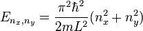
Since  and  can be interchanged without changing the energy, each energy level is at least twice as degenerate when  and  are different. Degenerate states are also obtained when the sum of squares of quantum numbers corresponding to different energy levels are the same.

Due to the restrictions of the electronic states , quantum dots exhibit interesting finite size effects which dominate much of the physics involved with them. The most noticable of these finite size effects are in fluorescence, where quantum dots in the form of nanoparticles fluoresce at specific frequencies depending on the size of the nanoparticles.

#2 Carbon Nanotubes

Quantum dots do not have to be nanoparticles however. We can create quantum dots by engineering quantum degnerate states of electrons in Single Walled Nanotubes (SWNTs) 

If we were to place a single-walled carbon nanotube (SWCNT) across an oscillating field bias, where the nanotube is bridged from source to drain, we can create a region inside the nanotube where an electron degeneracy has been induced (Fig-18).

Fig-18: A metallic SWNT is coupled via tunneling junctions to a source and drain contact. The chemical potential in the dot is adjusted by a gate voltage.

This introduced degeneracy in one region, the source, would then effectively generate a trapped electron-hole pair within the nanotube itself which has the benefit of having the effect of shielding the charges, thus functioning as a quantum dot. 

We would then have, the saturated absorption and thus a possibility to have stimulated emission of coherent photons. 

The electronic properties of carbon nanotubes are strongly influenced by the way the tubes are registered on a substrate. Quantum confinements in the form of periodic quantum-well (QW) structures are produced over the whole length of the nanotube and the size of the confined regions can be controlled by changing the mismatch between the tube and substrate.

The band-structure of the nanotubes can also be manipulated depending on the degree of mismatch between the nanotube and substrate so that is resembles a superlattice in which the bandgap energy is periodically modulated. In turn, this produces periodic modulations of the nanotube's electronic structure, which then appears as 1D multiple quantum dots.

Thanks to the extremely small size of the confined region, the energy level splittings observed for single walled carbon nanotubes can be very large (simulations suggesting to be around 300 meV), which means that the structure could operate as a quantum-dot system at room temperature operating with conventional electronics rather than just at ultra-low temperatures.

At low bias voltages the current can be turned off and on by varying the gate voltage. This is a consequence of the already mentioned, changing the gate voltage, which allows the transport of charge only for certain values of the electrochemical potential. 

Due to the band and spin degrees of freedom, each of the SWNT shells can carry multiple quantum dots, leading to a N-fold periodicity of the current as a function of the gate voltage. The magnitude of the current allows for conclusions concerning the structure of the ground states for a certain number of electrons in the dot.

At finite bias voltages, transport measurements serve as excitation spectroscopy, determining the energy levels but also the nature of the excited states. Because of the 1D nature of a SWNT in combination with the Coulomb interaction, the elementary excitations of the system can not be described as fermionic quasiparticles as for higher dimensional systems, but as bosons. We can calculate the transport properties of SWNTs quantum dots by using the so called reduced density matrix (RDM) formalism.

We can calculate, using simulation software such as Matlab, the current passing through the carbon nanotube quantum dot as a function of the gate and bias voltage which is plotted in Fig-19. We find the Coulomb Blockade regime with vanishing current at a point of avoidance crossing, which is characteristic of the charge carrying fermions, the electrons and holes, forming a coupled pair, which is a boson. Additionally we find excitation lines, where the current changes since new excited states become involved in transport.

Fig-19: Current passing through the SWCNT as a function of gate and bias voltage showing the Coulomb Blockade at the point of avoidance crossing

We can also use the RDM formalism to simulate the I/V characteristics of a Capacitive Coupled SWCNT system in this Coulomb Blockade Regime, in the frame of quantum-dot theory by the movement of the electrons and holes and observe the point of avoidance cross where they form a pair (with neutral voltage).

Fig-20: I/V curve of charge transport in the Coulomb Blockade regime. Such a curve, when observed experimentally, indicates quantum dot charge transport behavior in a SWCNT.

Meanwhile, using strain engineering in carbon nanotubes, the coupling of electron spin in carbon nanotube quantum dots with the nanotube’s nanomechanical vibrations can significantly affect the spin of an electron trapped on it. Moreover, in this way the electronic band structure of the carbon nanotube itself can be affected by the electron’s spin. The RDM theory is also well suited for the treatment of contacts that are polarized with respect to the spin and/or band degree of freedom. 

Likewise, if the quantum dot, structured inside the nanotube, was excited by a photon it would oscillate and create and effective field bias, which would have an effect of saturating the carbon nanotube in a field which would create a discrete set of limits on the absorption. Hence the concept of a carbon nanotube and/or quantum-dot based system of coherent laser emission and coherent laser absorption works in this regime. 

#3 Teraherz Radiation:

Studying new materials and new processes is good in the spirit of science and understanding, however the results from these investigations may create new frequencies in which we can employ lasers in particular the realm of practical means of Terahertz radiation generation and detection. Terahertz Radiation, THZ, which is the frequency band just between the far infrared and microwave regions of the EM spectrum (Fig-21) and is of key interest for opening up a new band of the EM spectrum for humankind to utilize in science and technology.

Fig-21: The Terahertz (THZ) Frequency Band and its relative position in the EM spectrum

Terahertz radiation is of key interest but more interesting still is the structuring of materials and systems that can utilize it. The fact that it is at the barrier between traditional optics technology and Microwave and RF technologies means that the end result will be a mixture of the two but also critically something entirely new that will be more than the sum of the parts. The fields of nanostructured materials and metamaterials are of key interest in this field.

It is not surprising therefore to see why there has been so much interest in the development of carbon nanotube and quantum dot based technologies for efficient laser tools, in particular in the field of saturable absorbers for Terahertz Q-switching, as well as more general applications in high-tech sensors, nanocrystal displays and solar photovoltaics to name but a few.

These 3 fields of applied physics: lasers, carbon nanotubes and quantum dots, are often treated exclusively of one another but this may not always remain that way as we begin to develop more refined physical models and engineer more efficient laser technologies.

All images are free for use and distribution under creative commons.

Article written and designed by MuonRay Enterprises Ireland - 2016