Image + Video Segmentation in Near-Infrared Using HSV Color Spaces with OpenCV in Python

Here I will be sharing a technique to perform a simple kind of image segmentation used to separate certain objects visible in the near-infrared and ultraviolet using the hue, saturation and value values (HSV) contained in the color space with OpenCV in Python. This is a useful tool in the processing of NIR images and video when we want to search for vegetation in an image using a defined threshold. Moreover, we can perform fast NDVI analysis on the examined region in the video clips. 

First of all we need to set up an idea of what we mean by segmentation. In this case it means to literally cut out an object that has a particular well defined colour in the image taken.

We should remember what we mean by colour itself in an image our brain, or a computer, "sees".

In a very real sense, we see with our mind's own programming, not with our eyes which merely sense changes in sensitivity across sensing elements, the cones in our eyes. For example consider sunlight shining on this apple

What is important to remember is that we do not see the red spectrum of light, but we see every other spectrum except that one! Every color except red is absorbed by the object, our eye sees this and sends a message to our brain. Our brain then labels this this as a red apple. 

This is a labeling procedure that our brains have developed with a dependence on the level of light exposed, not the intrinsic colour of the object. The best example of this dependent effect of light on color is seen when a colored lamp is put on something. If we had a red lamp and turned it on in a dark area, everything would appear to be red... that's because there's only red light to bounce off of it!

These special red street lamps were designed to stop harmful light pollution that can confuse and disturb the health and balance of nocturnal animals, such as bats, insects and even reptiles such as lizards and sea turtles. As we can see ourselves, otherwise green plant and black road appear red even though they would not appear red when radiated in balanced proportions of red green and blue light.

This principle is also true when we take photographs using a CCD sensor, which is equipped with a filter as to properly correlate with our own sense of vision, with some adjustments to sensitivity to light exposure, aperture size and shutter speed.

When the light of a scene enters the camera lens, it gets dispersed over the surface of the camera’s CCD sensor, a circuit containing millions of individual light detecting semiconductor photodiode sensors. Each photodiode measures the strength of the light striking it in Si unit called “lumens.” Each receptor on this sensor records its light value as a color pixel using a specific filter pattern, most commonly the Bayer filter.

A real image being focused and projected onto a CCD image sensor containing a colour filter. The Bayer Filter uses color filters and direct the individual colors red, green, blue onto individual pixels on the sensor, usually in an RGGB arrangement (i.e. 2X2 [RG;GB] ).

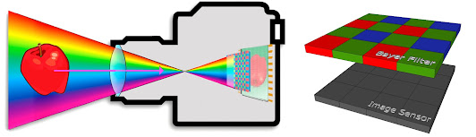
The camera’s image processor reads the color and intensity of the light striking each photoreceptor and maps each image from those initial values in a function called an input device transform (IDT) for the digital sensor information to be used to store a reasonable facsimile of the original scene in the form of raw data containing the color channels in separate channels for processing and colour processing. 

To display the image the raw data must be processed to have a color scale and luminance range to try and reproduce the color and light from the original scene. A display rendering transform (DRT) provides this mapping and are typically implemented in a form of preset ranges which are obtained using calibration standards, such as the SDR and HDR standards. Often raw data must be modified by standalone image processing software with the editor in command of controlling aspects such as contrast, gamma correction, histogram correction and so forth between the separate colour channels before we are given the final satisfactory image

With the RAW image data a process known as Demosaicing (which is also called de-Bayering in our case) is used to reconstruct a full color image, with RGB values at every pixel, from the incomplete color samples output from an image sensor overlaid with a color filter array (CFA).

When this bitmap of pixels gets viewed from a distance, the eye perceives the composite as a digital image. 

As discussed previously on this blog and showcased on my YouTube videos, I have been imaging individual plants and sections of vegetation in the near-infrared using drones for some time now. As I have shown, the plant material reflects very vibrantly in the near-infrared in the color channel which we associate with the colour red. Therefore if I want to segment the image to separate the plants from the background, using an infrared image, I can set the segmentation around the red color channel.

The individual color channels in an image, red, green and blue, can together form a group which we call a color space. In OpenCV in Python the color space is a tuple, a vector like object in the programming language. A color is then defined as a tuple of three components. Each component can take a value between 0 and 255, where the tuple (0, 0, 0) represents black and (255, 255, 255) represents white.

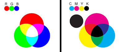
RGB (Red, Green and Blue) colour space is used normally to create colors that you see on television screens, computer screens, scanners and digital cameras.  RGB is often referred to as an 'additive colorspace.’ In other words, the more light there is on a screen means the brighter the image.

CMYK (Cyan, Magenta, Yellow and Black) is known as the 4-color process colors for printing. CMYK is considered a subtractive colorspace. May colour printers print with Cyan, Magenta, Yellow and Black (CMYK) ink, instead of RGB. It also produces a different color range. When printing on a 4-color printer, RGB files must be converted into CMYK color.

The RGB additive colour space vs the CMYK Subtractive Colour Space. As you may notice, there are certain RGB colors you see on your computer screen (or camera) that are unable to be duplicated with basic CMYK. Also notice that CMYK Colour can appear somewhat deeper than RGB combinations. This is part of the reason they are favored in printing.

The HSV (Hue, Saturation, Value) model, also called HSB (Hue, Saturation, Brightness), defines a color space in terms of three constituent components:

Hue, the color type (such as red, blue, or yellow): Ranges from 0-360 (but normalized to 0-100% in some applications)

Saturation, the "vibrancy" of the color: Ranges from 0-100%

Value, the brightness of the color: Ranges from 0-100%

Also sometimes called the "purity" by analogy to the colorimetric quantities excitation purity and colorimeric purity

The lower the saturation of a color, the more "grayness" is present and the more faded the color will appear, thus useful to define desaturation as the qualitative inverse of saturation

The HSV model was created in 1978 by Alvy Ray Smith. It is a nonlinear transformation of the RGB color space, and may be used in color progressions.

In HSV space, the red to orange color of plants in NIR are much more localized and visually separable.

Raw image of the HSV color space, stereographic projection of the surface on a circle

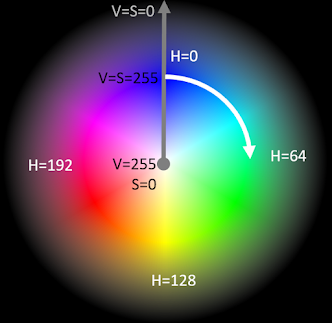
The HSV model is commonly used in computer graphics applications. In various application contexts, a user must choose a color to be applied to a particular graphical element. When used in this way, the HSV color wheel is often used. In it, the hue is represented by a circular region; a separate triangular region may be used to represent saturation and value. Typically, the vertical axis of the triangle indicates saturation, while the horizontal axis corresponds to value. In this way, a color can be chosen by first picking the hue from the circular region, then selecting the desired saturation and value from the triangular region.

Graphics artists sometimes prefer to use the HSV color model over alternative models such as RGB or CMYK, because of its similarities to the way humans tend to perceive color. RGB and CMYK are additive and subtractive models, respectively, defining color in terms of the combination of primaries, whereas HSV encapsulates information about a color in terms that are more familiar to humans: What color is it? How vibrant is it? How light or dark is it? The HSL color space is similar and arguably even better than HSV in this respect.

The HSV tristimulus space does not technically support a one-to-one mapping to physical power spectra as measured in radiometry. Thus it is not generally advisable to try to make direct comparisons between HSV coordinates and physical light properties such as wavelength or amplitude. However, if physical intuitions are indispensable, it is possible to translate HSV coordinates into pseudo-physical properties using the psychophysical terminology of colorimetry as follows:

Hue specifies the dominant wavelength of the color, except in the range between red and indigo (somewhere between 240 and 360 degrees) where the Hue denotes a position along the line of pure purples

If the hue perception were recreated, actually using a monochromatic, pure spectral color at the dominant wavelength, the desaturation would be roughly analogous to an applied frequency spread around the dominant wavelength or alternatively the amount of equal-power (i.e. white) light added to the pure spectral color.

The value is roughly analogous to the total power of the spectrum, or the maximum amplitude of the light waveform. However, it should be obvious from the equations below that value is actually closer to the power of the greatest spectral component (the statistical mode, not the cumulative power across the distribution.)

The saturation and value of the oranges do vary, but they are mostly located within a small range along the hue axis.This is the key point that can be leveraged for segmentation.

Segmentation of true color images in HSV color space can be applied to Near-Infrared photography in the imaging of the near-infrared reflectance of plants. 

By applying a threshold in the interpreted red band we can separate the vegetation, taken in the NIR, from the background. 

#threshold vegetation using the red to orange colors of the vegetation in the NIR

low_red = np.array([160, 105, 84])

high_red = np.array([179, 255, 255])

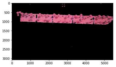
This is a fairly rough but effective segmentation of the Vegetation, in NIR, in HSV color space.

Going further we can process the selected region to form an NDVI in the region of interest. consider the NDVI taken broadly over the entire image:

Processing this image takes time, especially in RAW format, and in areas where there is more concrete and rock than vegetation much of the processing seems redundant as we usually do not care about NDVI scaling of rock.

Processing NDVI in the threshold region of interest meanwhile saves a lot of processing time and creates a more precise examination of NDVI with respect to the color key:

Here we see a video showcasing image segmentation for NDVI image processing using OpenCV in Python applied on Near-Infrared drone images and video.

This procedure is very useful for accurate scaling of NDVI in the region of interest, the vegetation of the image, and removing the background so as to focus on the NDVI of plant material only. The potential for detecting plants in an image or video is also a field of interest for us in plant exploration and detection in desert regions and for plant counting by techniques such as ring detection. It is hoped these developments will be useful in detecting rare or well hidden plant specimens in remote areas for plant population monitoring in deserts and mountains.

Notes:

OpenCV by default reads images in BGR format, so you’ll notice that it looks like the blue and red channels have been mixed up. You can use the cvtColor(image, flag) and the flag we looked at above to fix this:

Python Source Codes available on the following GitHub repository:

Coding available here: https://github.com/MuonRay/Image-Vide...