The Structure of Quantum Boltzmann Machines

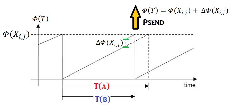
Previously we have thought about how we can think of a system of metaheuristic synchronization as a form of computational architecture, based on the path integral interpretation:

In the classical picture of such a network, which have local energy minima, we have a network made up of binary nodes (activations either 0 or 1), where the probability of achieving a coupling between the nodes would be set to 1 if and only if the connected nodes have the same activation, i.e A1=A2, i.e. the 2 activation levels have an allowed crossing. This has the effect of greatly limiting the nodal capacity of such systems.

To solve this problem we must relate our quantum mechanical system to equilibrium dynamics which will allow us to create a meta-heuristic representation of quantum diabatic behaviour which will induce the necessary condition of avoided crossing between nodes in the network.

Diabatic transitions can in fact be represented as a meta-heuristic algorithm therefore one need not go through the trouble of constructing a quantum computer to simulate annealing in the optimum way. For example, one thing that a metaheuristic, under the lens of the path integral interpretation of quantum mechanics, can do is a form of self-generating noise correction.

Using quantum dynamics, we can say that the Probability of a Diabatic Transition between 2 discrete energy levels E1 and E2 is given by the Landau-Zener Formula:

Where:

Where 

is the Landau-Zener Velocity for the perturbation variable q (where q is either a quantisation, i.e. a charge, of an electric or magnetic field, the length scale of a molecular bond, or any other perturbation to the system), and E1 and E2 are the energies of the two diabatic (crossing) states.

The quantity g is the off-diagonal coupling element of the two-level system's Hamiltonian that couples the crossing states, and as such it is half the distance between the two unperturbed eigenenergies at the avoided crossing, when E1 = E2.

We can write the transition probability as:

The adiabatic theorem in quantum mechanics therefore tells us, that as the difference between the energy states,Goes to 0, then the transition probability  goes to 1 (unity).

The adiabatic theorem in quantum mechanics therefore tells us, that as the difference between the energy states, α, Goes to 0, then the transition probability PD goes to 1 (unity).

This means that the quantised transitions between the energy states themselves are suppressed at the point of avoided crossing where 2 or more eigenvalues of the Hamiltonian cannot become equal in value.

This implies reversibility – i.e. no net work done, in a cyclic process.

In terms of thermal dynamics then we examine the transition probability in terms of the Energy Hamiltonian.

A quantum mechanical system is described by an eigenvalue problem.

                                      Hψn = e(n)ψn

where H is a Hermitian operator on function-space, ψn is an eigenfunction,

and e(n) is the corresponding (scalar) eigenvalue.

In this case H is the  Energy Hamiltonian, and the eigenvalue e(n) denotes the n-th energy level.

In Thermal Equilibrium Dynamics:

Since the occupation space can only be |0> or |1> for fermions,

An imaginary time path integral approach to thermal equilibrium dynamics can be performed by the fact that our canonical density operator

Is related to the time evolution operator in the Schrödinger scheme

By the analytic continuation of time, we define:

This is known in field theory as a Wick rotation from a Minkowskian to a Euclidean coordinate system used in field theory.

However, as we have shown, we can write the transition probability as a sum over histories in the path integral interpretation and furthermore can represent the path integral as a meta-heuristic signalling scheme in a neural network.

We can then unite the approach to achieve meta-heuristic synchronization with the adiabatic theorem of equilibrium dynamics which is where the longer the thermal system is allowed to transition to reach its final state in the time evolution from x0 to xt, the more likely it will have stayed in the ground state (or, said another way, the longer the system is allowed to run, the less likely there is to be random excitations, which basically translate to noise). 

Therefore, in order to reduce noise or error in such a system, all you need to do with a metaheuristic algorithm is to simply run the algorithm in the adiabatic fashion for a longer time. i.e. if you ran it for T = infinity, you'd be 100% accurate.

This is exactly the criterion for the standard metaheuristic signalling algorithm, as the signalling actions move towards the least signalling, and thus most energetically conservative, action possible.

This leads us to thinking of the metaheuristic concept of a neural network as being applicable to the classical Boltzmann Machine Framework which can overcome the problem of systems of binary nodes getting stuck in local energy minima by the addition of three key features:

• Stochastic activation function: the state a unit is in is probabilistically related to its Energy gap. The bigger the energy gap between its current state and the opposite state, the more likely the unit will flip states.
• Temperature and simulated annealing: the probability that a node is on is computed according to a activation function of its total weighted summed input divided by T. If T is large, the network behaves very randomly. T is gradually reduced and at each value of T, all the units' states are updated. Eventually, at the lowest T, units are behaving less randomly and more like binary threshold units.
• Contrastive Learning: A Boltzmann machine is trained in two phases, "clamped" and "unclamped". It can be trained either in supervised or unsupervised mode; this type of training proceeds as follows, for each training pattern:
1. Clamped Phase: The input units' states are clamped to (set and not permitted to change from) the training pattern, and the output units' states are clamped to the target vector. All other units' states are initialized randomly, and are then permitted to update until they reach "equilibrium" (simulated annealing). Then learning is applied.
2. Unclamped Phase: The input units' states are clamped to the training pattern. All other units' states (both hidden and output) are initialized randomly, and are then permitted to update until they reach "equilibrium". Then anti- learning (learning with a negative sign) is applied.

The above two-phase learning rule must be applied for each training pattern we feed into the network and for a great many iterations through the whole training set. Eventually, the output units' states should become identical in the clamped and unclamped phases, and so the two learning rules exactly cancel one another. Thus, at the point when the network is always producing the correct responses, the learning procedure naturally converges and all weight updates approach zero.

The stochasticity enables the Boltzmann machine to overcome the problem of getting stuck in local energy minima, while the contrastive learning rule allows the network to be trained with hidden features and thus overcomes the capacity limitations.

In the Boltzmann Machine framework, the state of the network is defined by an Energy Landscape. 

The global energy, , in a Boltzmann machine is identical in form to that of a Hopfield energy network:

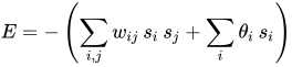
Where:

•  is the connection strength between unit  and unit .
•  is the state, , of unit .
•  is the bias of unit  in the global energy function. ( is the activation threshold for the unit.)

Often the weights are represented in matrix form with a symmetric matrix , with zeros along the diagonal.

The difference in the global energy that results from a single unit  being 0 (off) versus 1 (on), written , assuming a symmetric matrix of weights, is given by:

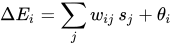
This can be expressed as the difference of energies of two states:

We then substitute the energy of each state with its relative probability according to the Boltzmann Factor (the property of a Boltzmann distribution that the energy of a state is proportional to the negative log probability of that state):

where  is Boltzmann's constant and is absorbed into the artificial notion of temperature .We then rearrange terms and consider that the probabilities of the unit being on and off must sum to one:

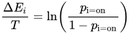
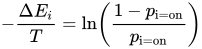
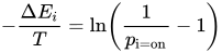
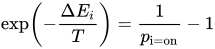
We can now finally solve for , the probability that the -th unit is on.

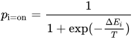
where the scalar  is referred to as the temperature of the system. 

The above function is of course a logistic sigmoid function, with the same form as the activation function in neural networks. 

Note: when T = 0 this gives a discrete step function for this probability and gives a uniform probability of 0.5.

The Boltzmann machine neural network is run by repeatedly choosing a unit and setting its state according to the above formula. After running for long enough at a certain temperature, the probability of a global state of the network will depend only upon that global state's energy, according to a Boltzmann distribution, and not on the initial state from which the process was started. 

This means that log-probabilities of global states become linear in their energies. This relationship is true when the machine is "at thermal equilibrium", meaning that the probability distribution of global states has converged. 

If we start running the network from a high temperature, and gradually decrease it until we reach a thermal equilibrium at a low temperature, we may converge to a distribution where the energy level fluctuates around the global minimum. This process is called simulated annealing.

It can be shown that after a certain time at fixed T, such networks reach a thermal equilibrium in which the probability of a given configuration of units is constant. Thus, while the precise state of the machine cannot be known, it is possible to reason about where it 'probably' is. 

For two such configurations A and B, suppose the respective energies are Ea and Eb and the associated probabilities P(A) and P(B) it can be shown that

That is, the probabilities follow a Boltzmann distribution. Note that since the sum of either the probabilities P(A) or P(B) equals unity (i.e. 1) then summing across all P(A):

where K is a constant depending on the interconnections, weights and temperature. Thus the state with the lowest energy has the highest probability.


If we gradually reduce T, we have a high probability of achieving a global minimum for the system energy. At high T we locate coarse minima, which are refined as T reduces (*see note). This is the criterion for simulated annealing. 

[ *Note: Another way to think about this is that when a system loses heat to its surroundings, the entropy of the system decreases and the entropy of the surroundings increases. Assuming the heat transfer occurs reversibly, then

                                         ΔS=∫δq/T 


where  T  is the temperature, and  δq  is negative for the system since the system is losing heat.

Hence the maximum change in entropy should occur at the lowest temperature. This maximum change in entropy gives us, equivalently, a perfectly uniform energy distribution, represented in terms of the logistic function being reduced to a completely convex energy basin with no bumps at all. Yet another way to picture such a state is in terms of the occupation of quantised energy levels, or rather the amount of time the machine stays at a particular energy level as thermal  energy is removed. Once T=0 the length of time the machine stays in the ground state, the global minimum, will be infinite. 

In reality, no ideal arrangement such as this can be reached with any real Boltzmann machine as there are always vacuum energy fluctuations that create the non-zero background temperature. Even a quantum computer working as a Boltzmann Machine at near-absolute zero would not have a truly uniform energy distribution such that you would be guaranteed to find the global minimum. ]


As in any neural network,  the units in the Boltzmann machine network are divided into 'visible' units, V, and 'hidden' units, H. 

The visible units are those which receive information from the 'environment', i.e. our training set is a set of binary vectors over the set V.

We hope to train the weights  such that when the input units are held at the appropriate 0,1 values ( clamped) the output units display the appropriate output pattern after annealing. 

This is done by performing the following cycle the necessary number of times;

The distribution over the training set is denoted ${\displaystyle P^{+}(V)}$.

As is discussed above, the distribution over global states converges as the Boltzmann machine reaches thermal equilibrium. 

We denote this distribution, after we marginalize it over the hidden units, as ${\displaystyle P^{-}(V)}$.

Our goal is to approximate the "real" distribution ${\displaystyle P^{+}(V)}$ using the ${\displaystyle P^{-}(V)}$ which will be produced (eventually) by the machine.

 To measure how similar the two distributions are, we use the Kullback–Leibler divergence, ${\displaystyle G}$:

${\displaystyle G=\sum _{v}{P^{+}(v)\ln \left({\frac {P^{+}(v)}{P^{-}(v)}}\right)}}$

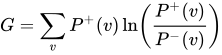
where the sum is over all the possible states of ${\displaystyle V}$. ${\displaystyle G}$ is a function of the weights, since they determine the energy of a state, and the energy determines ${\displaystyle P^{-}(v)}$, as promised by the Boltzmann distribution. Hence, we can use a gradient descent algorithm over ${\displaystyle G}$, so a given weight, ${\displaystyle w_{ij}}$ is changed by subtracting the partial derivative of ${\displaystyle G}$ with respect to the weight.

There are two phases to Boltzmann machine training, and we switch iteratively between them. One is the "positive" phase where the visible units' states are clamped to a particular binary state vector sampled from the training set (according to ${\displaystyle P^{+}}$). The other is the "negative" phase where the network is allowed to run freely, i.e. no units have their state determined by external data. Surprisingly enough, the gradient with respect to a given weight, ${\displaystyle w_{ij}}$, is given by the very simple equation (proved in Ackley et al):

${\displaystyle {\frac {\partial {G}}{\partial {w_{ij}}}}=-{\frac {1}{R}}[p_{ij}^{+}-p_{ij}^{-}]}$

where:

• ${\displaystyle p_{ij}^{+}}$ is the probability of units i and j both being on when the machine is at equilibrium on the positive phase.
• ${\displaystyle p_{ij}^{-}}$ is the probability of units i and j both being on when the machine is at equilibrium on the negative phase.
• ${\displaystyle R}$ denotes the learning rate

This result follows from the fact that at thermal equilibrium the probability ${\displaystyle P^{-}(s)}$ of any global state ${\displaystyle s}$ when the network is free-running is given by the Boltzmann distribution(hence the name "Boltzmann machine").

Remarkably, this learning rule is fairly biologically plausible because the only information needed to change the weights is provided by "local" information. That is, the connection (or synapse biologically speaking) does not need information about anything other than the two neurons it connects. This is far more biologically realistic than the information needed by a connection in many other neural network training algorithms, such as backpropagation.

The training of a Boltzmann machine does not use the EM algorithm, which is heavily used in machine learning. By minimizing the KL-divergence, it is equivalent to maximizing the log-likelihood of the data. Therefore, the training procedure performs gradient ascent on the log-likelihood of the observed data. This is in contrast to the EM algorithm, where the posterior distribution of the hidden nodes must be calculated before the maximization of the expected value of the complete data likelihood during the M-step.

Training the biases is similar, but uses only single node activity:

${\displaystyle {\frac {\partial {G}}{\partial {\theta _{i}}}}=-{\frac {1}{R}}[p_{i}^{+}-p_{i}^{-}]}$

Boltzmann learning is very powerful, but the complexity of the algorithm increases exponentially as more neurons are added to the network. This makes learning is impractical in general Boltzmann machines. However, learning in Boltzmann Machines can be made quite efficient in an architecture called the "Restricted Boltzmann machine" or "RBM" which does not allow intralayer connections between hidden units. 

The hidden nodes in an RBM are not interconnected as they are in regular Boltzmann networks. Once trained on a particular feature set, these RBM can be combined together into larger, more diverse machines, such as polymer rings of different nodes.

Because Boltzmann machine weight updates only require looking at the expected distributions of surrounding neurons, it is a plausible model for how actual biological neural networks learn.

Boltzmann learning is statistical in nature, and is derived from the field of thermodynamics. It is similar to error-correction learning and is used during supervised training. In this algorithm, the state of each individual neuron, in addition to the system output, are taken into account. In this respect, the Boltzmann learning rule is significantly slower than the error-correction learning rule.

Restricted Boltzmann Machine learning is particular interest when considering so-called Polymer Rings and the means used to simulate them. Polymer rings are essentially compact Gaussian chains of individual Restricted Boltzmann machines subject to strong interactions with neighboring chains due to the presence of topological constraints. 

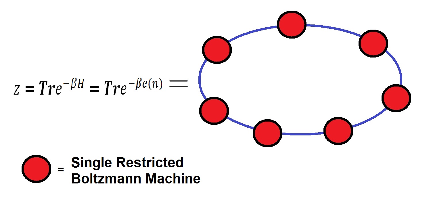
Therefore, using imposed constraints on individual single Boltzmann Machines, one can perform ring polymer simulations that use a Restricted Boltzmann Machine to model the dynamics of networks much faster than using standard unconstrained Boltzmann machines. 


A constraint can be established by means of restricting communication between each individual Boltzmann machine by a search procedures, such that only the nearest neighbors to each individual Boltzmann machine is activated by its closest neighbors and ignores everything else. Such a search procedure, based on nearest neighbors, could be accomplished using a variety of already established methods.


By the path-integral interpretation of machine signalling, any system with sufficient discontinuous pas-coupling should therefore have a self-generating property of meta-heuristic behaviour.

In such a case the nodes involved with carrying out the neural activity are themselves already active in an ad-hoc synchronization procedure which organizes the nodes such that the least action principle of signalling can occur between the nodes.

In such a case, we need not even think about this in the sense of performing quantum evolution in terms of path integrals on polymer chain simulations, as doing a metaheuristic simulation should be functionally equivalent as a quantum path integral in this view.

This is the reasoning for how it is possible to use metaheuristics to solve NP-hard problems. Quantum computing of this kind, although interesting in and of itself, has very broad applications in any field involving a networked topology, which spans a huge realm of empirically observed behaviour in both organic and inorganic signalling systems.

Viewing Meta-Heuristic Synchronization using the Path Integral Interpretation

We can investigate and compare the probabilistic representation of the path integral theory with the description of a metaheuristic signalling algorithm as a system of discontinuous pas-coupling.

Discontinuous pas coupling can occur in a variety of system. It is especially important in the field of wireless signalling, such as using radio waves, microwaves or optical light sources such as LEDs and Lasers to transmit data. In such a system, where information packets are transmitted and received, you have quite naturally a discontinuity based on external and internal natures of the transmission infrastructure, interference, decoherence and obstructions.

So lets say we are interested in discontinuous pas coupling, as the strategy to achieve synchronization. Within such a system you might have arbitrary network conditions, individual delays and additionally you will have appropriately to receive packets.

This means that there is a random chance that the signal that is transmitted is not going to be received. This has all to be taken into account and, as discussed in our article on metaheuristics, is when why use metaheuristic algorithms that contain randomization elements along with the nature of the transmission power law function in order to achieve and guarantee synchronization between oscillating nodes.

Let us take our oscillators running on a unit circle in phase-space. The oscillators represented on a circle in phase space. To achieve synchronization, the oscillators runs clockwise on the circle until it passes the threshold. Whenever it passes the threshold, it will emit a signal pulse, with some probability, Psend. When the oscillators are coupled, they will adjust their individual rates, or periods, of signalling to match with one another (encroaching closer together on the unit circle in phase-space) to achieve synchronization under a time evolution.

Each oscillator will adjust its period of signalling according to our signalling activation function, which is, under the signalling field representation, a phase function:

The function evolves linear over time, until it reaches a threshold value, defined by the vector weights, X i,j, which are translated into coupling strengths under the powerlaw-based metaheuristic as explained previously.

When the threshold is reached, a single oscillator fires the signal pulse and then resets its phase. If no coupling occurs, the oscillator will pulse with a period, T(A). T is effectively the encoded time remaining until the next signal pulse.

When a phase-coupling occurs between oscillators, when an oscillator receives a pulse it will increment its phase function by an amount that itself depends on its current value and the change induced by the weights of the received signal. The oscillator will then pulse with a new period, T(B):

This means that an oscillator, that is in the lower half of the phase-space circle, will jump forward, and an oscillator that is in the upper half, will jump backwards in the circle in phase space. This is the main concept of a self-organizing update function, which brings the 2 oscillators in phase with one another and thus coupled.

The resemblance of the unitary time-evolution operator in quantum mechanics to the monotonically decreasing signalling function is obvious in their respective mathematical forms:

Moreover, like the unitary time-evolution operator, the signalling algorithm is readily compatible with Lagrangian mechanics in the same way as the unitary time-evolution operator which are inherently used for discrete particles each with a finite number of degrees of freedom.

The classic Lagrangian is written as the difference of the kinetic and potential energy density of a particle.

The potential energy density of the particle is a field density, such as an electromagnetic field density in generalised coordinates V(q).

Since v=p/m, the kinetic energy can of course be written in terms of momentum, p,  which is more relevant for what we are describing.

The abbreviated action S0 is defined as the integral of the generalized momenta along a path in the generalized coordinates q

in our ad-hoc system of synchronization coupling, the momenta will be replaced by Psend and integrated over the time domain (dt) in the path it takes to achieve synchronization. This leads to the total Signalling Action,Sf, being represented as the phase of each path being determined by ∫ Psend dt, for that trajectory.

The frequency of signalling is then, as an oscillation in phase-space:

Using this in the path-integral view we can represent the synchronization procedure as:

In this convention, the signalling action, Sf, which is a real operator is defined as being essentially characteristic of the physical and environmental parameters of the system – namely the light absorption coefficient and the power law over the distance by which it is subject to.

Since each deviation from the path of least action is, just like in the case with a quantum particle, proportional to the action imparted on the system, the signal activation function will activate with a frequency proportional to the action. Therefore, the path of least possible action, which occurs during complete internal synchronization, should have the lowest frequency of signal function activation.

An increase in frequency of signal activation indicates a deviation from the path of least possible signalling action.

Therefore, when using any metaheuristic algorithm, when looking for any deviations, i.e. faults, between the coupled oscillators when internal synchronization is achieved we should just have to look for any changes in the frequency of the signalling between the different nodes.

What do I mean by this?

I mean that when an interaction occurs with our signalling model, the deviation leads to a deviation from the path of least signalling action to achieve synchronization, as we have imparted our own equivalent signalling action, Sf, onto the system.

This causes an initial synchronization collapse. However, the action, Sf, imparted towards the path will lead to an increase in the rate of cycles, i.e. an increase in the signalling action away from the least signalling action, and thus an increase in the probability of achieving synchronization with neighbours again.

In effect, internal processes are stimulated under any signalling action, increasing their state of energy, which is “unfavoured” - unfavoured as the increasing energy state will itself drive the quantised nodes, which have a discrete threshold, that make up the system to spend more energy and thus increase cycling which overall increases the probability that the area under interaction will be synchronized with its neighbours again. Therefore the system is able to restore itself back to synchronization. 

For example, we can have an experimental system of coupled oscillators, as described above, that achieve synchronization through emitting signals to one another over a time series. In the beginning, our 2 (or more) oscillators can be viewed as having similar signals over the time series but are out of phase with each other. As before, the update function is designed to change the period of emitting the signal pulse,(i.e.  T(A) , to T(B))
for each of the oscillators until they achieve synchronicity. In effect we are aligning the time sequences of the 2 signals. 

Dynamical Time Warping, DTW is a technique used for measuring the similarity between two sequences of data in terms of their distances and allowing to find the optimal path to align them in phase. Therefore, it can be a way to represent the degree of coupling between 2 oscillators, signalling in a time series. 

A great many measures of “distance” between 2 different time series of signals have been developed, sometimes called "clustering distances". These are used in many fields involving clusters of data in a signal such as in image analysis, signal processing and machine learning.  

The 3 main types of clustering distances are Euclidean, Manhattan and Minkowski distances:

We shall be using Euclidean Distance as our preferred distance metric, for the simple reason that for our universal power-law signalling algorithm the distance between any 2 nodes is a Euclidean distance using Cartesian coordinates. 

So in the Euclidean distance the sequences are aligned "one-to-one" with the ith point on one time series aligned with the ith point on the other. This itself produces a poor measure of similarity between 2 signals.


In DTW, non-linear alignments (i.e. out of phase sequences T(A) and T(B) ) can be made, thus better measures of similarities between sequences can be made:

In DTW we compare the 2 time series while accounting for the distances, or "warping" (shown above as the coloured lines between T(A) and T(B) ) between the non-linear alignments by dynamic programming. The warp is then resolved by either adding samples or deleting samples.

The warping between the 2 series is calculated by constructing an M x N matrix, which we shall call P.

For P = M x N 

M is the length of one time series: X = X1,...XM

N is the length of the other time series: Y = Y1,...YM

The Euclidean distance is now made up of 2D vectors, Xi and Yj, with each point in the matrix position being p(i,j).

p(0,0) is classified as 0 

p(i,0) and p(0,j) are classified as infinity

The optimum path is calculated by minimizing the degree of warping that occurs in the diagonal paths through this matrix. This is done by comparing, in each matrix cell (i,j),  the time series up to position i in X and position j in Y by the following recursion: 

Which gives us the minimum coordinate distance for each element as: 

By this recursion method we achieve the total warping path, W.

In terms of use in the path integral interpretation of synchronization, the total warping path is equivalent to the total Signalling Action,Sf.

Defining the total warping path, W = W1,...Ws,....Wk. 

The points of the Matrix the warping passes across are 

Ws=(is,js), s=1,2, …,k. 

d(Ws) is an individual distance between corresponding elements of series T(A) and T(B).



The total warping between sequence T(A) and T(B) is therefore:

Which is our DTW recursive function.

To isolate the path of least action, or least warping, some restrictions need to be applied to the recursive function. These include the following:

• Monotonic condition: the path will not turn back on itself, both the i and j indexes either stay the same or increase, they never decrease.
• Continuity condition: the path advances one step at a time. Both i and j can only increase by at most 1 on each step along the path.
• Boundary condition: the path starts at the bottom left and ends at the top right.
• Warping window condition: a good path is unlikely to wander very far from the diagonal. The distance that the path is allowed to wander is the window width. For example, a given warping path, W, should be within the distance between (j = i+W) and (j=i-W)
• Slope constraint condition: The path should not be too steep or too shallow. This prevents short sequences matching too long ones. The condition is expressed as a ratio p/q where p is the number of steps allowed in the same (horizontal or vertical) direction. After p steps in the same direction is not allowed to step further in the same direction before stepping at least q time in the diagonal direction.

In this way the number of possible paths is greatly reduced to only those of particular interest.

In the diagram below we show how DTW give a optimal path (arrangement) to minimize the total distance between the two series, a test series and a reference series. 

The above is a reference set compared against one node. The same is repeated for all the trained ones in the network.

For a particular oscillator (test) in comparison to the rest of the system (reference) the system is 100% synchronized over time when we have a perfect diagonal along the grid generated between the test sample and reference.

By then exposing the synchronized system (i.e. the reference) to a non-synchronized light source, or by introducing a new oscillation, we can induce a deviation from the path of least action of the system that leads to a initial synchronization collapse. This is represented by the path warping in the DTW picture.

However, the collapse, or warp, itself increases the rate at which the disturbed oscillators signal to one another by the metaheuristic procedure, i.e. increases the energy consumption of the system. However this itself in turn increases the probability of restoring synchronization and the state of least energy consumption, least action, possible for the system and so the diagonal path through the grid can be restored.

Constructing Neural Networks from Multiple Synchronized Oscillators

Using this information in our view of meta-heuristics we can go further and incorporate this into neural network structures under the path integral interpretation.

The system of synchronized coupled oscillators forms the neural network structure. We can then reduce the input vectors to an input signalling action oscillating at a certain input frequency in the complex plane,which passes through the network, for example under sigmoidal or other Gaussian analog activation functions, in our path integral interpretation. 

This then gives an output signalling action, or "class", of certain nodes in the network which will now carry a period of oscillation, characteristic of the input signal as interpreted by the neural network. The weights the input vector acts on in the neural network picture are then replaced by the paths in the sum over all possible taken in the time-evolution to achieve synchronization within the network.

I represent this construct in the diagram below, in which I have created a Radial Basis Function synchronized neural network in Matlab which receives a signal and creates an output response characteristic of this input, broadened by the k-number of paths of sigmoidal activation function signalling within the network:

We then say there is an output “class” of internal node signalling action in the network from being stimulated by an external signalling action, in which sense our input signalling action is interpreted as a “class” by the nodes after passing through the neural network.

It is perhaps important to note that the signalling action towards the generation of nodal output classes is clearly not the core function of the neural network and is merely ancillary to it. By this I mean that the vector inputs and their associated weights cause action on the network but in this case are not in fact forming the network structure itself. 

In summary, a network structure can be formed, independently, by the time-evolution of the discontinuous pas-coupling generated by the meta-heuristic nature of the internal signalling which can in principle be described using a path integral interpretation.