The term computer has had many different incarnations of meaning over the past 100 years. From the human computers at Los Alamos, the room-sized valve computers to modern semiconductor computers, the word computer had become far more generalized than its original definition.
A computer is a logic filing system functioning within the parameters of a particular hardware.
Modern computers use programs, themselves merely sophisticated filing systems, functioning in the parameters of the Boolean logic of computer hardware, which is a series of semiconductor chips and electrical components.
The apparent complexity of computation is, in reality, sending and retrieving a series of previously written instructions. Computer programs need to execute functions by calling on a series of header files written in a particular language to work through a continuum of instructions to perform any task. these header files are themselves made up of instructions, written in a computer language, which itself is a substitution of a more fundamental and arcane machine code, ultimately in binary 0s and 1s.
Computation as we know it, i.e. a Turing Machine, must use this method if it is constructed with switching elements be they valves or transistors.
Some problems which Turing Machines are used to solve are nondeterministic, i.e. a program that is, or depends on, a random number generator running in polynomial or exponential timescales. these timescales are such that they are equal to or grater than the number of operations (arithmetic, sorting, matchings, ect).
The operations of this class, known as P operations (P for Polynomial time) are the most tractable problems in complexity theory and are at the foundation of all complex computations. Due to them being deterministic it is possible for a computer to know how long it takes to solve these problems and so it is no surprise that most functions of a computer use algorithms that break down most hard problems into P operations, such as the case of the halting problem which defines the Turing-complete model of computation.
Due to the use of a a random number generator, solutions to the algorithm will be nondeterministic at such timescales. These are NP operations. Although any given solution to such a problem can be verified quickly by approximation or by randomization (as in Monte Carlo simulations) there is no known efficient way using a computer to locate a solution in the first place. The most notable characteristic of NP-complete problems (where every element is NP) is that no fast solution to them is known because the timescales involved are completely random. NP-complete problems could take anywhere between 10 seconds and 10 trillion years to solve, even if they are relatively simple.
However, the solution becomes deterministic if checked by a deterministic Turing subroutine that solves a different problem that uses polynomial time excluding the time within the subroutine. Intuitively, a polynomial-time reduction proves that the first problem is no more difficult than the second one, because whenever an efficient algorithm exists for second problem, one exists for the first problem as well. These are NP-hard problems.
Most NP-Complete and NP-hard problems are optimization and search problems, such as the travelling salesman problem or Langton's ant, Langton's Loops, Turmites and Turing-type cellular automatons in general.
The K-SAT problem plays a most important role in the Theory of Computation (NPcompleteproblem) The setup of the KSAT Computation (NP complete problem). The setup of the K-SAT problem is as follows
• Let B={x1, x2, …, xn} be a set of Boolean variables.
that satisfies all clauses simultaneously, i.e.
More advanced versions of these algorithms require large timescales to work with, which is not much use for search results for the here and now. Therefore we sometimes need the computational equivalent of the educated guess. It turns out there is such a thing. They are called heuristics.
(performed in CERN ROOT Code)
Field of view of Kepler spacecraft, trained on a patch of more than 150,000 stars near the constellation Cygnus, trails Earth as both orbit the sun. One common false positive Kepler is trained to notice is an eclipsing binary star behind one of Kepler's target stars; the background light blocked by such an eclipse can mimic the periodic dimming that Kepler uses to identify planets passing in front of its target stars.
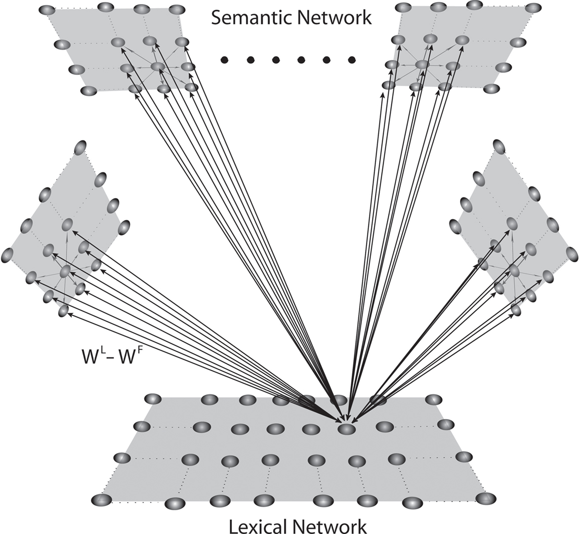
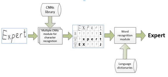
More generally, neural networks can be used in full image reconstructions and shape recognition as well as in error analysis. These programs have some level of self correction and can learn in a sense. However they are not self-sufficient as "training" programs must be fed to the program before it can be at a level where it can correct itself.
Such A.I. metaheuristics may resemble global optimization problems similar to classical problems such as the travelling salesman, ant colony or swarm optimization, which can navigate through maze-like databases. The solutions, although not completely optimal, are far more useful than a typical heuristic would be. If used in parallel processing, such heuristics display machine learning which do make assumptions on the task being solved. This means that error analysis is possible with these heuristics.
Metaheuristics are also used in Monte Carlo method simulations to create global optimization, which are widely used in physics and science in general to solve problems. One such problem is Simulated Annealing.
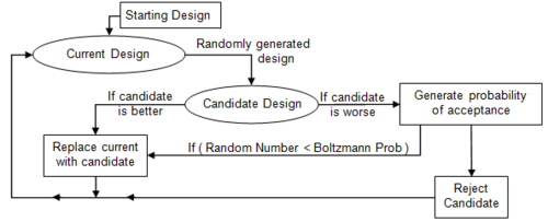
Simulated annealing copies a phenomenon in nature--the annealing of solids--to optimize a complex system. Annealing refers to heating a solid and then cooling it slowly. Atoms then assume a nearly globally minimum energy state. In 1953 Metropolis created an algorithm to simulate the annealing process. The algorithm simulates a small random displacement of an atom that results in a change in energy. If the change in energy is negative, the energy state of the new configuration is lower and the new configuration is accepted. If the change in energy is positive, the new configuration has a higher energy state; however, it may still be accepted according to the Boltzmann probability factor:
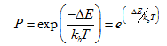
where is the Boltzmann constant and T is the current temperature. By examining this equation we should note two things: the probability is proportional to temperature--as the solid cools, the probability gets smaller; and inversely proportional to --as the change in energy is larger the probability of accepting the change gets smaller.
When applied to engineering design, an analogy is made between energy and the objective function. The design is started at a high “temperature”, where it has a high objective (we assume we are minimizing). Random perturbations are then made to the design. If the objective is lower, the new design is made the current design; if it is higher, it may still be accepted according the probability given by the Boltzmann factor. The Boltzmann probability is compared to a random number drawn from a uniform distribution between 0 and 1; if the random number is smaller than the Boltzmann probability, the configuration is accepted. This allows the algorithm to escape local minima.
As the temperature is gradually lowered, the probability that a worse design is accepted becomes smaller. Typically at high temperatures the gross structure of the design emerges which is then refined at lower temperatures.
Although it can be used for continuous problems, simulated annealing is especially effective when applied to combinatorial or discrete problems. Although the algorithm is not guaranteed to find the best optimum, it will often find near optimum designs with many fewer design evaluations than other algorithms. (It can still be computationally expensive, however.) It is also an easy algorithm to implement.
The Metropolis-Hastings Algorithm generates sample states of a given thermodynamic system.
The Metropolis–Hastings algorithm can draw samples from any probability distribution P(x), which can be from the Boltzman Distribution, Fermi-Dirac Distribution or Bose-Einstein Distribution just provided you can compute the value of a function Q(x) which is proportional to the density of P.
The lax requirement that Q(x) should be merely proportional to the density, rather than exactly equal to it, makes the Metropolis–Hastings algorithm particularly useful, because calculating the necessary normalization factor is often extremely difficult using Bayesian Probability Statistics.
The Metropolis–Hastings algorithm works by generating a sequence of sample values in such a way that, as more and more sample values are produced, the distribution of values more closely approximates the desired distribution, P(x).
These sample values are produced iteratively, with the distribution of the next sample being dependent only on the current sample value (thus making the sequence of samples into a Markov chain). Specifically, at each iteration, the algorithm picks a candidate for the next sample value based on the current sample value. Then, with some probability, the candidate is either accepted (in which case the candidate value is used in the next iteration) or rejected (in which case the candidate value is discarded, and current value is reused in the next iteration)−the probability of acceptance is determined by comparing the likelihoods of the current and candidate sample values with respect to the desired distribution P(x).
Simulated Annealing in terms of Metaheuristics
Simulated Annealing is a stochastic method for optimization problems but can also be considered as a metaheuristic search method for the approximate solution of optimization problems. A typical example is the problem of finding a sequence of different processing steps of a production, so that the orders as quickly as possible without each block to the machine can be carried out. If we denote the set of all possible order with S , then a * x from S to find with minimal execution time c (x *) . If you imagine the cost function c: S -> R as a landscape before, in the high values c (x)a raised dot at the point x mean, it is therefore the aim of finding a deep valley as possible.

Starting from a random starting point
x0 examined simulated annealing random solutions
Y in the neighborhood of the current solution
x . Y is more than
x , that is, applies
c (y) <C (x) , then
y is accepted as the new solution. In the cost landscape of a downhill path is of
x by
y taken. Applies the other hand
c (y)> c (x) , the path leads from
x by
y that is uphill, the
y still accepted as a new solution - but only with a certain probability, called the acceptance probability. This ability to accept deteriorations, the process may leave local valleys and advance to the global minimum, as indicated in the following figure.
As acceptance probability for a candidate y at current solution x is usually (- (c (y)-c (x)) / tn) exp is selected. It is tn the so-called temperature with increasing step number n to 0 goes. Minor deterioration D = c (y)-c (x)> 0 are thus more acceptable than larger, even with increasing n, thus decreasing temperature degradations are rarely accepted. If a solution y not accepted, a new candidate is y ' from the neighborhood randomly selected.

The method is based on a physical model for cooling processes ('annealing') in molten metals, which depends on the temperature control, the material can build up especially favorable structures during solidification. When initially high temperatures many deteriorations are accepted, the process moves usually quickly from the starting point off in the long run, the threshold for acceptance of deterioration is higher, the process comes to rest.
The order of visited solutions forms an inhomogeneous Markoffkette and it can conditions for the convergence to an optimal solution are given.
We can go further with these simulation and imagine particles which could operate under the principles of quantum mechanics in such algorithms.
Metaheuristics and Quantum Computing
Quantum computers use entangled particles as qubits. In superconducting Jospehson junctions, the electrons form Cooper Pairs which can undergo quantum tunneling through the superconducting material and the normal conducting or insulating material.
By thinking about quantum computation in the same way as we think about classical probabilistic computation then we can make active progress in discovering how we can use a quantum computer and how we can use it to perform algorithms such as simulated annealing.
Quantum theory is the language which describes how systems, on the order of Planck's Constant, evolve in time. Thus we are led, in our most fundamental physical theories, to descriptions of systems which are quantum mechanical. These systems, like everything else, can be either analog or digital
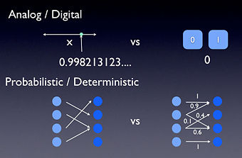
A digital system is a system whose configurations are a finite set. In other words a digital system has configurations which you might label as zero, one, two, etc, up to some final number. Now of course, most digital systems are abstractions. For example the digital information represented by voltages in your computer is digital in the sense that you define a certain voltage range to be a zero and another range to be one. Thus even though the underlying system may not be digital, from the perspective of how you use the computer, being digital is a good approximation.
Analog systems, as opposed to digital systems, are the ones whose configurations aren't drawn from a finite set. Thus, for example, in classical physics, an analog system might be the location of a bug on a line segment. To properly describe where the bug is we need to use the infinite set of real numbers.
Digital and analog are words which we use to describe the configurations of a physical system (physicists would call these degrees of freedom.) But often a physical system, while it may be digital or analog, also has uncertainty associated with it.
Thus it is also useful to also make a distinction between systems which are deterministic and those which are probabilistic. Now technically these two ideas really refer to how a systems configurations change with time. But they also influence how we describe the system at a given time.
A deterministic system is one in which the configuration at some time is completely determined by the configuration at some previous time. A probabilistic system is one in which the configurations change and, either because we are ignorant of information or for some more fundamental reason, these changes are not known with certainty. For systems which evolve deterministically, we can write down that we know the state of the system. For systems which evolve probabilistically, we aren't allowed to describe our system in such precise terms, but must associate probabilities to be in particular configurations.
There is often a confusion between analog systems and probabilistic systems. The first refers to degrees of freedom or configurations. The second refers to how a system changes in time, or what we can predict about it once we make a measurement on it.
Let's consider a single bit. In probability theory, we can describe a bit as having a probability p of being 0, and a probability 1-p of being 1. But if we switch from the 1-norm to the 2-norm, now we no longer want two numbers that sum to 1, we want two numbers whose
squares sum to 1. (I'm assuming we're still talking about real numbers.) In other words, we now want a vector (α,β) where α
2 + β
2 = 1. Of course, the set of
all such vectors forms a circle:
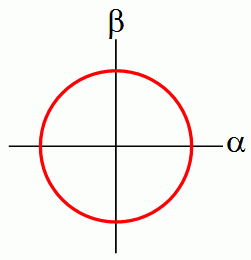
The theory we're inventing will
somehow have to connect to observation. So, suppose we have a bit that's described by this vector (α,β). Then we'll need to specify what happens if we
look at the bit. Well, since it
is a bit, we should see either 0 or 1! Furthermore, the probability of seeing 0 and the probability of seeing 1 had better add up to 1. Now, starting from the vector (α,β), how can we get two numbers that add up to 1? Simple: we can let α
2 be the probability of a 0 outcome, and let β
2 be the probability of a 1 outcome.
But in that case, why not forget about α and β, and just describe the bit
directly in terms of probabilities? Ahhhhh. The difference comes in how the vector changes when we apply an operation to it. In probability theory, if we have a bit that's represented by the vector (p,1-p), then we can represent any operation on the bit by a
stochastic matrix: that is, a matrix of nonnegative real numbers where every column adds up to 1. So for example, the "bit flip" operation -- which changes the probability of a 1 outcome from p to 1-p -- can be represented as follows:
\left(\begin{array}%20p\\1-p\end{array}\right)=\left(\begin{array}1-p\\p\end{array}\right))
Indeed, it turns out that a stochastic matrix is the
most general sort of matrix that always maps a probability vector to another probability vector.
It turns out that the set made of deterministic and probabilistic really has another member, and this member is quantum. For probabilistic systems we describe our configuration by a set of positive real numbers which sum to unity, while for quantum systems these numbers are replaced by amplitudes, complex numbers whose absolute value squared sum to unity. A quantum system is as simple as that: a system whose description is given by amplitudes and not probabilities.
Hence, in the complex plane, the possible amplitudes which sum to unity are in a superposition of 0 and 1 as represented by the following Argand diagram:

Physicists like to represent qubits using what they call "Dirac ket notation," in which the vector (α,β) becomes

. Here α is the
amplitude of outcome |0〉, and β is the amplitude of outcome |1〉.
Therefore, with digital systems we should have 3 different types of bit information configuration, classical bits which are deterministic, probabilistic bits which are stochastic and quantum bits which are unitary.
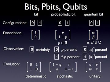
Therefore the concept of a quantum bit is similar to a probabilistic bit in that the value is government by a output percentage but this is not a probability anymore, it is an amplitude of a probability for which of the coherent superposition of a quantum observable's eigenstates (alpha and beta) jumps to, which is given by a probabilistic law such that the probability of the system jumping to the state is proportional to the absolute value of the corresponding linear combination squared.
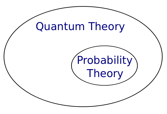
In a sense, we can consider probability theory as a subset of quantum theory as far as computation is concerned.
Many body systems of entangled states in quantum circuits are studied using
powerful numerical techniques, some of which were developed under the broad scope of quantum information theory without specifying a particular physical framework for building the circuit, i.e. superconducting, optical, quantum spin, ect.
The Density Matrix Renormalization Group (DMRG) is one such technique which applies the Numerical Renormalization Group (NRG) to quantum lattice many-body systems such as the Hubbard model of strongly correlated electrons, forming Cooper pairs in superconductors say, as well as being extended to a great variety of problems in all fields of physics and to quantum chemistry.
The DMRG algorithm has attracted significant attention as a robust quantum chemical approach to multireference electronic structure problems in which a large number of electrons have to be highly correlated in a large-size orbital space. It can be seen as a substitute for the exact diagonalization method that is able to diagonalize large-size Hamiltonian matrices. It comprises only a polynomial number of parameters and computational operations, but is able to involve a full set of the Slater determinants or electronic configurations in the Hilbert space, of which the size nominally scales exponentially with the number of active electrons and orbitals, allowing a compact representation of the wavefunction.


In applications to quantum lattice systems, such as in superconducting quantum circuits, DMRG consists in a systematic truncation of the system Hilbert space, keeping a small number of important states in a series of subsystems of increasing size to construct wave functions of the full system. In DMRG the states kept to construct a
renormalization group transformation are the most probable eigenstates of a reduced
density matrix instead of the lowest energy states kept in a standard NRG calculation. DMRG techniques for strongly correlated systems have been substantially improved and extended since their conception in 1992. They have proved to be both extremely accurate for low-dimensional problems and widely applicable. They enable numerically exact calculations (i.e., as good as exact diagonalizations) on large lattices with up to a few thousand particles and sites (compared to less than a few tens for exact diagonalizations).
Originally, DMRG has been considered as a renormalization group method. Recently, the interpretation of DMRG as a matrix-product state has been emphasized. From this point of view, DMRG is an algorithm for optimizing a variational wavefunction with the structure of a matrix-product state. This formulation of DMRG has revealed the deep connection between the density-matrix renormalization approach and quantum information theory and has lead to significant extensions of DMRG algorithms. In particular, efficient algorithms for simulating the time-evolution of quantum many-body systems have been developed.
Simulating large quantum circuits with a classical computer requires enormous computational power, because the number of quantum states increases exponentially as a function of number of qubits. The DMRG was introduced to study the properties of relatively large-scale one-dimensional quantum systems, as this method corresponds to an efficient data compression for one-dimensional quantum systems. By applying the DMRG method to quantum circuit simulation, simple quantum circuits based on Grover's algorithm can be simulated with a classical computer of reasonably modest computational power.
In such simulations, we are dealing with reversible quantum computing circuits, which requires a special type of bit, called an ancilla bit. In this scheme the ancilla bit must be prepared as a fixed qubit state used for input to a gate to give the gate a more specific logic function. These can be either prepared as computational basis of random numbers, possible solutions or guess heuristics.
DMRG works well on all physical systems with low ground state entanglement.
However QMA problems yield highly entangled ground states! To do DMRG models we would need less entangled ground states which would be an automatic restriction of proof & verifier circuit!
Our only choice therefore would be to just accept classical proofs and classical verifier circuits, i.e. restriction of all problems to NP.
QMA: The quantum version of NP – the class of problems where “yes” instances have a quantum proof which can be efficiently checked by a quantum computer
We are interested in the spectral gap for each instance independently not in the promise gap between “yes” and “no” instances.
To make registering locally accessible time must be encoded in spatial location of qubits, by the time-dependent Hamiltonian.
Realization of Hamiltonian is made by adding a control register; implement a control unit, a
“head”, of propagating qubits in the circuit.
A finite control unit consists of a finite number of qubits pi that the condition of the machine are in a Hilbert space.
An infinite memory of which a finite part is used: this is an infinite set of qubits mi serving in a Hilbert space and memory for the machine.
On the basis of the density matrix, rho, we can re-express the concept of observation as a probability.
The probability of finding a particular eigenstate, |k>, in the quantum register in a given initial state, |phi> can be calculated as
We can, in a similar way, get the expectation value of a quantum measurement, as
A is the observable with the matrix of the system.
This is nothing more than the average of individual probabilities of energy configuration values.
The energy expectation value will not be used further in this text, but it is important as an educational example for the NMR quantum computer which was the first use of this technology based on the quantum energy states of molecules under a particular spin state.
The NMR quantum computer, using a powerful external magnetic field to align molecules, made measurements using uniform microwave pulses and, at a measurement, then gets the average of all possible energy configurations, which correspond to whether the spins are aligned with or against the external field.
Nuclear spins are advantageous as qubits, since they have very good isolation from mechanisms that can lead to decoherence. This leads to long relaxation times. Moreover spins can be manipulated by  pulses to effect appropriate unitary operations.
Tthe Hamiltonian of a spin

particle in constant magnetic field

along

, is given by
where  is the Larmor precession frequency and is typically of the order of 100MHz. Spins of different nuclei are distinguishable by their different Larmor Frequencies. Spins of same nuclei in a molecule can have slightly different Larmor frequencies owing to different chemical shifts (typically in 10-100ppm), hence rendering them distinguishable
It is convenient to use the pictorial Bloch Sphere representation
 where
where  is the angle from the z-axis and
  is the azimuthal angle. Under the constant magnetic field, the Bloch vector precesses about the z-axis.
Application of
field of amplitude

at

, makes the spin evolve under the transformation

where

is the pulse-width.
This gives a rotation by an angle proportional to the product of tpw and !1 about an axis in the

plane determined by the phase
. E.g. A pulse of

and

cause rotation about

by

, i.e.

(90), where as a pulse of same width but with phase causes

.
Using rotations about
and

, any arbitrary single qubit

can be implemented
Using the spin-spin coupling Hamiltonian it is possible to impliment a 2-qubit C-NOT Gate.
Physically is can be said that, a spin \feels" an additional magnetic field due to neighboring spins causing a shift in Larmor frequency A line selective

pulse at frequency,

can then be used as a CNOT operation. This causes spin ip of the second qubit, via Rabi oscillation, only when the first qubit is 1.
Two qubit Control Not Gate
There are several hurdles in implementing NMR quantum computation. First of all it is extremely difficult to address and read individual spins. A large number of molecules must be present to produce measurable signals.The number of molecules in the 7-bit NMR quantum computer built by IBM for example had a magnitude of 10^18 molecules Hence the NMR signal is an average over all the molecules' signals.
The quantum register used for the implementation is a organic molecule consisting of five 19 F and two 13 C nuclei, i.e. a total of seven spin-1/2 nuclei, as shown below:
But quantum computation requires preparation, manipulation, coherent evolution and measurement of pure quantum states, so using a statistical mixture above a certain number of molecules eliminates the coherence required for quantum computation meaning that NMR quantum computation was limited using such approaches to move beyond a few 10s of qubits.
Regardless of the technology, with an observed quantum register we get, after detection, a new initial state given by
Note that we in our observation of a quantum register we project the state vector at a subspace of the Hilbert space:
Considering a 3-qubit quantum register
We first calculate the odds of calculating the values {0.....7} of the quantum register
After detection, the new initial state will then be
In the Matlab software, this quantum registering procedure can be implemented
function x = measure(x, k)
dim = length(x); % the number of basis states
n = log2(dim); % number of bits in the register
if nargin == 1, k = [0:n-1]; end;
for i = 1:length(k)
prob_0 = probability_0(x, k(i));
if prob_0 > rand
% observed a ’0’
x = apply([1/sqrt(prob_0) 0; 0 0], k(i), x);
else
% observed a ’1’
x = apply([0 0; 0 1/sqrt(1-prob_0)], k(i), x);
end;
end;
dynamical correlation model, Canonical Transformation Theory, that is tailored to efficient incorporation into large-scale static (or strong) correlation. In CT model, higher-level dynamic correlations are described from a unitary cluster many-body operator,
eA |Ψ0 ⟩ = (1 + A + 1/2 A2+...) |Ψ0 ⟩, where A†=-A.
In a related picture, we can view eA as generating an effective canonically transformed Hamiltonian HCT that acts only in the active space, but which has dynamic correlation folded in from the external space, where
HCT = e-A H eA = H + [H,A] + 1/2 [[H,A],A] + ....
A central feature of the canonical transformation theory is the use of a novel operator decomposition, both to "approximately" close the infinite expansions associated with the exponential ansatz and to reduce the complexity of the energy and amplitude equations, resulting in a scalable internally-contracted multireference algorithm (o(N6)).

CT algorithm is designed to be incorporated into large-scale static correlation, which is assumed to be handled with modern powerful diagonalization techniques, such as density matrix renormalizatoin group (DMRG).
Expanding on these models generates the quantum analog of the Turing machine:
The resulting Hamiltonian has a spectral gap above ground states. Finding the ground state (energy) is NP-hard. Therefore other techniques must be developed to transform the initial ground state of a quantum system to the final ground state.
Adiabatic Quantum Computation (AQC) is a universal model for quantum computation which seeks to transform the initial ground state of a quantum system into a final ground state encoding the answer to a computational problem.
By using Josephson junctions, like those present in Superconducting Quantum Interferencd Devices (SQUIDs) as qubit elements in a quantum computer chip, such as constructed by NIST in America and D-Wave Systems in Canada, the algorithms used in Simulated Annealing can be extended into Quantum Annealing, where solutions exist that allow for the effects of quantum mechanics to tunnel through the maxima in probability distributions.
You can have an analogy of the annealing by imagining you put a block of ice in a cup, and you turn up the heat to make it melt. Your goal is to make the ice melt as slowly as possible, so that when you have your cup of water, you have absolutely zero vibrations or waves. You can imagine that by some super-heating method that if the ice cube were to instantaneously turn into water, there would be waves going everywhere since the water would be rushing out to the walls of the cup. What you want to do is heat it slowly so that this never happens, not even in the slightest. Your tolerance is, say, 99%. If your ice cube is an Adiabatic Quantum Computer, AQC, vibrations in the final state (the water) are "excitations", which basically mean errors and, thus, giving you wrong answers. They may be close, but they wouldn't be optimal.
So you have this system of connected qubits in SQUID form is that you prepare this system with a magnetic field that is going a certain way. You then you slowly turn off your initial state while slowly turning on your final state. So basically you're going through a mixed state of initial and final energy, though by the end there will be basically no initial parts of the problem left in the state and you're left only with the final state. An alternative way is to start with both states on, but have the initial state be much, much stronger than the final part of the state, and then slowly turn off the very large, initial state. If you find this confusing, take a look at this equation

H stands for Hamiltonian, which is just a name for a matrix that defines the total energy state of the system. The three terms, you'll notice, can be grouped into two terms really. the big Z and X are referring to the spin matrices. So in terms of this equation, your initial state is governed by the last term, and your final state is governed by the first two terms. The spin matrices show the change from the X-basis state to the Z-basis state. When you prepare your initial system of qubits, you put them all into the X-spin state and then anneal to the Z-spin state. Imagine that h and J are much, much smaller than K initially. When you anneal, you slowly turn off K so that when you're done, you're only left with whatever is in the first two terms. This is how the annealing process works.
Now in order to anneal properly so that you get the correct answer, you need to be sure you're giving it enough time to settle without excitations. The above equation is time-dependent, or more specifically, the h, J, and K terms are time-dependent. Now the adiabatic theorem will tell you that unless you run for t = infinity, you will not reach 100% accuracy. Still, we can get close. Even 90% isn't so bad, given that you're quickly reaching a somewhat optimal solution.
In terms of the math and quantum mechanics, your state vector always needs to be in the lowest eigenstate of the Hamiltonian. An eigenstate, in linear algebra, would be equivalent to an eigenvector of some matrix. If you're familiar with quantum mechanics, you'll know that particles can only be in discrete energy states. The energy of this system would be the Hamiltonian, which is a matrix, and the lowest energy state is given by the lowest eigenvector of this Hamiltonian. If you wanted to know the actual energy level, that would be the lowest eigenvalue that goes with the aforementioned eigenvector/eigenstate. Now when you're annealing, you always want to be in the ground state. This is why you must move slowly, because if you move too quickly you are imparting energy into the system, causing excitations and jumps to higher energy levels. This is not good because that's where your errors come from.
Once you've gone through the annealing process, you'll wonder a few things. How do I know I've gotten the right answer? How much time should I have given my program to run? Is there a way to do some on-the-fly error correction?
Well, you will have to do tests on your problem to know if you got the right answer. Typically if you're solving an NP-complete problem, you can check if your solution is correct pretty quickly. Still, you will want to run the computation many times until you put that particular algorithm to use in any serious case. There are measures for this as well, however, and they have to do with tracking the actual energy of the Hamiltonian, finding its ground state eigenvector, and then comparing it with what your qubit state actually is. The inner product of the two will show you your error. Note that this can only be done theoretically, as you wouldn't be able to track your quantum state without observing it (and therefore, changing it).
On the fly error correction is also possible in a simulation of an AQC. Let me back up here. There is an idea that you can write some numerical software so that you can simulate the annealing process and come up with a time-scheme for your particular algorithm. Since it's a simulation, you have access to your state vector at all times and you can measure the predicted error according to the mathematics. You can do on-the-fly error correction by looking at the measures of error and correctness, and then adjusting your annealing timesteps accordingly. Take a look at this graph:

This is what is called the eigenspectrum of a 1-qubit simulation. Basically, it is showing you the energies through the annealing time for 1 qubit. Look at the x-axis as time. The bottom curve is the ground state, and the upper curve is the first excited state. Notice how at some point you will get that the two curves are very close. This is a crucial point, because the smaller this energy "gap" is, the more likely it is that the state of the system will jump to this higher energy state instead of stay in the ground state. Clearly this is a time where you want to move very slowly. Conversely, when the energy gap is very large, you can move rather quickly without worrying if you're going to jump to a higher state since it's pretty unlikely. You can come up with a time-scheme that means you go very fast up until that n = 0.5 point, and start to go much more slowly until you've passed the small-gap threshold.
By applying the concept of adiabatic transitions to maxima and minima in simulated annealing, it is possible to examine how particles could quantum tunnel between such maxima and minima.
Adiabatic curves exist between the maxima and minima of isotherms in thermodynamic plots. Such adiabatic transitions are, on the level of quantum mechanics, happen as competing a process where quantum systems tunnel between energy barriers.
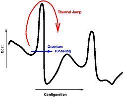
In superconductor materials, electrons form in pairs of particles, forming bosonic quasi-particles called Cooper pairs. These bosons can form entangled states with one another at temperatures where the thermal oscillations of the individual pairs are quenched, dropping the potential energy barrier to form such entanglement, therefore allowing the effects of quantum entanglement take over. This effectively forms a Bose-Einstein Condensate, where all particles are at the lowest possible energy level.
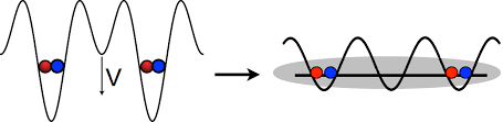
By incorporating superconducting materials in Josephson Junction circuits such that quanta can tunnel between the energy barriers experienced at the boundary between the superconductor and insulator or normal metal in an adiabatic mode, quantum switching elements can be created, and hence quantum computers, can be built around such models.

Schematic representation of a level anticrossing. The energies of two quantum states |Ψ1〉 and |Ψ2〉 localized in distant wells can be fine-tuned by applying a smooth additional potential.
(A) Before the crossing, the ground state is |Ψ2〉 with energy close to E2(s); i.e., for s- < sc, we have that E1(s-) > E2(s-), so that |GS(s-)〉 = |Ψ2〉.
(B) After the crossing, the ground state becomes |Ψ1〉 with energy close to E1(s); i.e., for s+ > sc, we have that E1(s+) < E2(s+), so that |GS(s+)〉 = |Ψ1〉.
The ground states before and after the crossing have nothing to do with each other. At a certain interval of s close to sc, the anticrossing takes place and the ground state is a linear combination of |Ψ1〉 and |Ψ2〉.
The nature of these models is based on the Hamiltonian operator derived from the adiabatic theorem.
The main idea behind quantum adiabatic algorithms is to employ the Schrödinger equation

AQC algorithms involve the specification of a time- dependent Hamiltonian,
This Hamiltonian has three important functions:
(1) The initial Hamiltonian, Hi ≡ H(0), encodes a ground state that is easy to prepare and that is used as the initial state for the quantum evolution.
(2) The driving Hamiltonian, ˆ hdriving(t), is responsible for mediating the transformation of the initial ground state to any of other state.
(3) The final Hamiltonian, ˆ Hf ≡ ˆ H(τ), is prob- lem dependent and its ground state encodes the solu- tion, |ψsolutioni, to the computational problem.
In the ideal case of a process being fully adiabatic, evolution under ˆ H(t) will keep the quantum state, |ψ(t)i, in the ground state of ˆ H(t) throughout 0 < t < τ. If this condition is met, the final state at t = τ should coin- cide with the ground state of the final Hamiltonian, ˆ Hf, i.e., |ψ(τ)i = |ψsolutioni, if the process is adiabatic. The measurement at t = τ will provide the solution to the computational problem.
Sombrero Adiabatic Quantum Computation (SAQC) Hamiltonian.
The goal of AQC algorithms is that of transforming an initial ground state |ψ(0)i into a final ground state |ψ(τ)i, which encodes the answer to the problem. This is achieved by evolving the corresponding physical sys- tem according to the Schr¨odinger equation with a time- dependent Hamiltonian ˆ H(t).
The AQC algorithm re- lies on the quantum adiabatic theorem [25–35], which states that if the quantum evolution is initialized with the ground state of the initial Hamiltonian, the time prop- agation of this quantum state will remain very close to the instantaneous ground state |ψg(t)i for all t ∈ [0,τ], whenever ˆ H(t) varies slowly throughout the propagation time t ∈ [0,τ]. This holds under the assumption that the ground state manifold does not cross the energy lev- els which lead to excited states of the final Hamiltonian. Here, we denote by ground state manifold the first m curves associated with the lowest eigenvalue of the time- dependent Hamiltonian for t ∈ [0,τ], where m is the degeneracy of the final Hamiltonian ground state.
Conventionally the adiabatic evolution path is the lin- ear sweep of s ∈ [0,1], where s = t/τ:
H(s) = (1−s)Htransverse + sHf. (3) ˆ
Htransverse (see Eq. 9 below) is usually chosen such that its ground state is a uniform superposition of all possible 2n computational basis vectors, for the case of an n−qubit system. Here, we choose the spin states {|qi = 0i,|q = 1i}, which are the eigenvec- tors of ˆ σz i with eigenvalues +1 and -1, respectively, as the basis vectors.
AQC initial Hamiltonians conventionally have a uniform superposition as ground state. A divergence from this practice can be made by introducing a simple form of heuristics: the ability to start the quantum evolution with a state which is a guess to the solution of the problem.
As preparing an arbitrary initial non-degenerate ground state for adiabatic evolution is not a trivial task, we focus on easy to prepare initial guesses that consist of one of the states in the computational basis. The strat- egy proposed builds initial Hamiltonians such that the initial guess corresponds to the non-degenerate ground state of the initial Hamiltonian, as it is required by AQC. Additionally, this ground state would be non-degenerate. Let us denote the states of the computational basis of an N qubit system as |qNi|qN−1i···|q1i ≡ |qN ···q1i where qn ∈ {0,1}. The proposed initial Hamiltonian, whose ground state corresponds to an arbitrary initial guess state of the form |xN ···x1i, can be written as ˆ
Hi =
N X n=1
xn ˆ I + ˆ qn(1−2xn) =
N X n=1 ˆ
hxn, (5)
where each xn is a boolean variable, xn ∈{0,1}, while ˆ q ≡ 1 2(ˆ I − ˆ σz) is a quantum operator acting on the n-th qubit of the multipartite Hilbert space HN ⊗HN−1 ⊗ ···⊗Hn ⊗···⊗H1. The operator ˆ qn is given by ˆ
qn = ˆ IN ⊗ ˆ IN−1 ⊗···⊗(ˆ q)n ⊗···⊗ ˆ I1, (6)
where ˆ q is placed in the nth position and the identity operators act on the rest of the Hilbert space. The states constituting the computational basis, |0iand |1i, are eigenvectors of ˆ σz with eigenvalues +1 and −1, and therefore they are also eigenstates of the oper- ator ˆ q with eigenvalues 0 and 1 respectively. The logic behind the initial Hamiltonian in Eq. 5 then is clear: if xn = 0, then ˆ hxn=0 = ˆ qn but in the case of xn = 1, then ˆ hxn=1 = ˆ I − ˆ qn.
a sig- nificant amount of progress has been made towards the design of final Hamiltonians for different computation- ally intractable problems such as NP-complete problems.
construction of the final Hamiltonian for an NP- hard problem of interest in biology, such as in the protein folding problem, a result of the famous Thermodynamic Hypothesis of protein Folding, which consists of finding the minimum energy configuration of a chain of interacting amino acids in a lattice model.
The hypotheisis is that the native fold of a globular protein is usually assumed to correspond to the global minimum of the protein’s Gibbs free energy.
The protein folding problem can be thus analyzed as a global optimization problem, with global maxima and minima.
 3D ribbon model of the protein ribonuclease A. Beta strands are arrows and alpha-helices are spirals. The disulphide bonds can from only after the protein folds into its native conformation. The native folding of the protein could be modeled using global optimization models using Adiabatic Quantum Computation.
The main idea behind Sombrero Adiabatic Quantum Computation (SAQC) is to introduce heuristics in AQC, and having the possibility of restarting a failed AQC run from the measured excited state. In order to prepare an arbitrary state from any of the 2N possible basis states from the computational basis of the N qubit system, we propose an initial Hamiltonian, ˆ Hi (see Eq. 5), in such a way that the desired initial guess state is the non-degenerate ground state of the designed initial Hamiltonian. The initial Hamiltonian is diagonal in the computational basis, and so is the final Hamiltonian for the case of classical problems such as the NP-complete problems, e.g., random 3-SAT. Since both, the initial and final Hamiltonians are diagonal, connecting them via a linear ramp as is usually done in CAQC (see left panel) will not lead the quantum evolution towards finding the ground state of the final Hamiltonian. To maintain the initial Hamiltonian uniquely and fully turned on at the beginning, t = 0, and the final Hamiltonian uniquely and fully turned on at the end of the computation, t = τ, we introduce a driving Hamiltonian whose time profile intensity has a “sombrero-like” shape (see right panel) is such a way that it only acts during 0 < t < τ. Two examples of functions with this functional form are presented, where hat1(s) = sin2(πs) and hat2(s) = s(1−s). A desired feature of our algorithmic strategy is the possibility of introducing heuristics, and not that of introducing non-linear paths. The latter has been proposed previous publications [8, 36, 37], but here is employed as a consequence of the algorithmic strategy.
For SAQC, the time-dependent Hamiltonian can be written as: ˆ Hsombrero = (1−s) ˆ Hi + hat(s) ˆ Hdriving + s ˆ Hf. (4)
We want the non-degenerate ground state of the ini- tial Hamiltonian ˆ Hi to encode a guess to the solution, and the driving term, ˆ Hdriving, to couple the states in the computational basis. The function hat(s) is zero at the beginning and end of the adiabatic path; therefore ˆ Hdriving acts only in the range s ∈ (0,1) in a “sombrero mexican hat- like” time dependence
Implementation of an SAQC algorithm either in
parallel (for 2 or more quantum computers) or in
serial (for single quantum computers).
The algorithm begins by choosing a state from the computational basis. For each chosen initial state, an initial Hamiltonian is prepared based on a random or classical heuristic in a continuous cycle of operations.
Next, an ideal time constraint is chosen, assuming a CAQC protocol will be run, which is to be used as a reference to run the SAQC protocol twice as fast.
If only one AQC computer is available, we can cheat here by having a probabilistic model of SAQC to run two separate adiabatic protocols instead of one, in serial mode. Once the first SAQC calculation is finished, one can efficiently check whether or not the result is a solution. In case that it is not a solution, one can submit an additional calculation, either randomly selecting another initial guess state or using the measured excited state.
If we use the measured excited state we are using a
“quantum heuristic” since the outcome of the near-adiabatic quantum evolution is used to refine the initial guess state for further use of the protocol.
In the case of having several adiabatic quantum computers at hand, one can do the same initial procedure of selecting guesses, but now submitting a different guess to a different node and running on each node twice as fast.
With this goal in mind, the viability of this approach has been explored along with the needed modifications to the conventional AQC (CAQC) algorithm. By performing a numerical study on hard-to-satisfy 6 and 7 bit random instances of the satisfiability problem (3-SAT), heuristic approaches are possible.
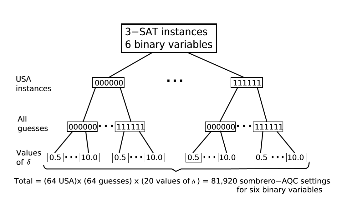
Scheme for 6 binary variables SAQC calculations. We generated 26 3-SAT unique satisfying assignment (USA) instances (first branching), each having as its only solution one of the 26 possible assignments. All 26 instances have a different state as solution, i.e. there is no chance for repeated instances. For each instance, we computed minimum-gap values associated with all possible settings of SAQC.
Of all possible guesses (second branching), using 20 different values of δ ∈{0.5,1.0,...,10.0} (third branching).
The same scheme was applied to 7 binary variable 3-SAT USA instances (not shown) for a total of (128USA)×(128guesses)×(20values of δ) = 327,680 SAQC settings
The performance of the particular algorithm proposed is largely determined by the Hamming distance of the chosen initial guess state with respect to the solution. Besides the possibility of introducing educated guesses as initial states, the new strategy allows for the possibility of restarting a failed adiabatic process from the measured excited state as opposed to restarting from the full superposition of states as in CAQC. The outcome of the measurement can be used as a more refined guess state to restart the adiabatic evolution. This concatenated restart process is another heuristic that the CAQC strategy cannot capture.
By using a decentralized, quantum swarm AI, it may be possible to simulate emergent behavior aswell, such as Langton's ant, which could see the rise of quantum-based simulated intelligence which could go so far as to create realistic cellular automatons on a computer.
The use of sophisticated metaheuristics on lower heuristical functions may see computer simulations which can select specific sub routines on computers by themselves to solve problems in an intelligent way. In this way the machines would be far more adaptable to changes in sensory data and would be able to function with far more automation than would be possible with normal computers.
Moreover, it may be possible to use metaheuristics to perform error correction on software using neural networks by comparing the optimized problem solving in a quantum computer with the regular programming software of a regular computer. Since regular computers are not quantum mechanical, they must be programmed classically. However, by using quantum metaheuristics it may be possible to perform optimization problems using Artificial intelligence on a quantum computer and then compare to the command line architecture in a piece of conventional software on a classical computer, which may be too complex to modify or to check for errors using human software engineers.
It may become routine that to design large software, rather than use a team of engineers to design a single piece of large software and to do multiple tests, revisions and redistribution, quantum optimization problems will be run though a machine instructed to do a particular task and the software will be designed around such optimizations.
Computer chips could even be designed to be superconducting and quantum compatible in a factory or laboratory and classically operating in conventional computer equipment. In this way, optimization and programming could be done on the chips in a factory or lab to search for any possible errors that could arise in designing software. After which the chips would be used in conventional computers for their particular tasks. Quantum computers may well find their place in industry more than anywhere else, designing AI optimized software around computer chips.
Metaheuristics will depend on the existence of the software to be designed around a particular problem solution, hence its optimization of solving the solution comes from a search of such solutions in a network. such searches could utilized neural network algorithms and would be the simulation of artificial intelligence. However for true artificial intelligence another step must be made, one that goes back to the fundamental concept of a heuristic being a solution to optimization. The program must recognize that some heuristics under certain circumstances are good, while others are bad.
Such an intelligence would require automated planning, and would be essentially the computer controlling its own strategies, for use at certain times, based on predictive modelling. It would use these plans in automated strategies which would attempt to find the right method by selecting a sequence of learned metaheuristics in a given situation.
This would be no longer metaheuristics, it would be hyperheuristics. the fact that this species of heuristics depends on learned metaheuristics means that it depends on feed-back learning. Hence this would be a machine that, after an initial amount of metaheuristic training would eventially begin to learn itself in a sulf-sustained way. In this way, a hyperheuristical machine would start out in a metaheuristical state and after a period of training it would "evolve" into a hyperheuriscal machine and begin a learning feedback.
How could it accomplish this? Hyperheursics could be to have the computer make changes to the theoretical global optimization model in response to learned behavior which would crate a sustained loop between learning and decision making so that it would have complete automated planning in response to an input. An adaptive planning machine would have to be a hyperheuristical machine.
As we have seen, the limitations of global optimization models can be improved through the technique of Adiabatic Quantum Computation. Therefore the most advanced type of heuristic possible would have to be based on quantum computer technology.
Approximations of such AI come in the form of Memetic Algorithms which evolve under the concept of Universal Darwinism. These programs are evolved on the basis of the transference of information.
applications include (but are not limited to) training of artificial neural networks,[17] pattern recognition,[18] robotic motion planning,[19] beam orientation,[20] circuit design,[21] electric service restoration,[22] medical expert systems,[23] single machine scheduling,[24] automatic timetabling (notably, the timetable for the NHL),[25] manpower scheduling,[26] nurse rostering and function optimisation,[27] processor allocation,[28] maintenance scheduling (for example, of an electric distribution network),[29]multidimensional knapsack problem,[30] VLSI design,[31] clustering of gene expression profiles,[32] feature/gene selection,[33][34] and multi-class, multi-objective feature selection.[35]
Alan Turing was not only the founder of modern computer technology, based on switching elements be they valves, transistors, molecular states or quantum spin states, but he also wrote the first paper on Artificial Intelligence, AI.
Turing also thought we may instead change our concept of thinking, however in reality the study of artificial intelligence has not formulated any fundamental theories of the nature of thought processes. in the 50 years since Turing, AI procedures, with very few exceptions, have gone more towards accumulating known methods and strategies, i.e. heuristics and running through them rapidly with group force methods rather than going through developing knew methods in how to diagnose and navigate problems.
In this sense heuristics have dominated AI at the expense of other methods, for example diagnostic and navigation methods using neural networks and models based on insect navigation for example. The reason heuristics have been used is because computer technology has largely been focused on the development of larger machine memories, to store large amounts of heuristics and programmed commands. the heuristic and command programs are, in reality, theories written in an arcane notation, designed to be executed by a machine. The nature of the machine itself executing the file is rendered irrelevant because of the fact that the program itself is stored in a highly ordered, layered fashion in computer memory, which is a spectator not a participant in virtually all theoretical models of AI.
The only known exceptions are based on advanced forms of insect navigation or neural network simulation, which are sometimes modeled from theories based on the neurobiology of squids. However these models often come nowhere near the level of complexity seen in living neurological systems. A bee, an insect with quite sophisticated navigational intelligence, for example has around 900,000 neurons, humans have 90 billion. The largest neural networks ever created by chains of supercomputers simulate, at best, only around 1% of the human brain.
In this sense, ideas such as"the singularity" is a very misleading subject, based more on fiction than on real science. There may very well be a revolution in what is commonly labelled "AI", but unless there is going to be a severe change in diagnostic and navigation of problems in computing then the field on AI will continue to be based on group force heuristics, error correction and new techniques of object-oriented computer programming, such that it could at best generate a so-called "oracle", but not a "genies" or "sovereign" machine that some of the literature predicts.
It is important to understand that by machine intelligence we are always, if we are being honest, talking about the structure of a computer program, as the operations will always be a series of instructions of what the program can to do and what lower level programs need to be selected to complete the circuitry generated by the program firmware, which only then influences the hardware. Therefore we actually need a theoretical basis to generate intelligent programming, which requires new techniques in heuristics, self correction and new forms of object-oriented programming which, in my opinion, has not been developed. Simply looking at a simple Moore's law plot is not enough, even ignoring the fact that it is beginning to level off with the limits of silicon being reached.
The Turing Test is the most commonly cited method of testing how intelligent a machine program is by having the human user communicate with both a machine and another human via computer screens and the user being unable to judge which is the human, based on answered questions that the user asks.
Summarized in the Venn Diagram below, we might also see the Turing Test as more accurately a test of human intelligence with respect to human behavior rather than to purely test machine intelligence
Here we see that the computer could easily have a set of heuristics which it would use to implement responses to answers in order to generate positive results. Moreover, if trained, the computer could use metaheuristics in response to patterns of questions which, under its training exercises, it knows that will give positive results.
At such a point asking whether or not the machine is "thinking" will be meaningless - it will be obvious that it processes intelligent action based on a selected strategy, not a complex theoretical model where the computer has been programmed to contemplate.
The real barrier therefore is to have the computer then generate predictive models based on a theory of human intelligence, which is something which we are no where near completing.
However, it would be naive to expect machine intelligence to emerge based on raw computation power alone as although the mathematical model and the computational power used to solve problems will have been developed in a gradual process, the selection of which models work best will have been selected over the models that had failed, which would be promptly deemed obsolete and eliminated. It would simply make no sense for a computer program to chose a possible solution unless it was based on a predictive model that was the best one, for all time every time. The problem is we don't have the best predictive model for how intelligence arises, least of all for individual human beings.
Moreover, to have a complex model of intelligence that works for all time neglects the fact that the most complex dynamical systems are highly sensitive to slight changes in initial conditions, such in the case of a sensory data input. This is of course concerning the field of Chaos Theory. Chaos would clearly be inherent in even the most ideal predictive model of intelligence, even more so based on its complexity.







![[Competitive learning scheme]](http://vv.carleton.ca/~neil/neural/neuron9.gif)
![[Neural weightings for letter `A']](http://vv.carleton.ca/~neil/neural/neuron10.gif) The example above is so simple that it is in fact a complete waste of a neural net, but it does demonstrate the principle. The output neurons of this type of network do not require thresholds because what matters is highest output. A more useful example would be a 5x7 pixel grid that could recognize letters. One could have 26 neurons that all share the same 35 pixel input space. Each neuron would compute the probability of the inputs matching its character. The grid on the left is configured to output the probability that the input is the letter A. Each tile in the grid represents a link to the A neuron.
The example above is so simple that it is in fact a complete waste of a neural net, but it does demonstrate the principle. The output neurons of this type of network do not require thresholds because what matters is highest output. A more useful example would be a 5x7 pixel grid that could recognize letters. One could have 26 neurons that all share the same 35 pixel input space. Each neuron would compute the probability of the inputs matching its character. The grid on the left is configured to output the probability that the input is the letter A. Each tile in the grid represents a link to the A neuron.![[Network that recognizes digits from 0 to 9]](http://vv.carleton.ca/~neil/neural/neuron11.gif) Training these pattern recognition networks is simple. Draw the desired pattern and select the neuron that should learn that pattern. For each active pixel, add one to the weight of the link between the pixel and the neuron in training. Subtract one from the weight of each link between an inactive pixel and the neuron in training. To avoid ingraining a pattern beyond all hope of modification, it is wise to set a limit on the absolute weights. The Recog character recognition program uses this technique to learn handwriting. It is a Windows application that can quickly learn to distinguish a dozen or so symbols. The network to the right was created by Recog to recognize the digits from 0-9.
Training these pattern recognition networks is simple. Draw the desired pattern and select the neuron that should learn that pattern. For each active pixel, add one to the weight of the link between the pixel and the neuron in training. Subtract one from the weight of each link between an inactive pixel and the neuron in training. To avoid ingraining a pattern beyond all hope of modification, it is wise to set a limit on the absolute weights. The Recog character recognition program uses this technique to learn handwriting. It is a Windows application that can quickly learn to distinguish a dozen or so symbols. The network to the right was created by Recog to recognize the digits from 0-9.